This report summarises the impact of reducing the flow temperature of a gas-condensing boiler under controlled conditions at the Salford Energy House.
The impact of reducing the flow temperature of a domestic gas condensing boiler was measured at whole-house level under controlled conditions at the University of Salford Energy House test facility.
The study found that:
- Lowering the boiler flow temperature reduced space heating gas use eg, lowering it from 80 degrees to 60 degrees saved 12% of gas used to heat the house
- However, it also slowed heat-up rates and lowered internal air temperatures e.g. when lowered from 80 degrees to 60 degrees, heat-up times in the morning went from 23 minutes to 37 minutes.
- The reductions in gas use measured are primarily due to increased boiler efficiencies rather than reductions in internal air temperature.
Money Saving Boiler Challenge
Our campaign aims to help over one million households change their combi boiler settings to save energy.
Executive Summary
The impact of reducing the flow temperature of a domestic gas condensing boiler was measured at whole-house level under controlled conditions at the University of Salford Energy House test facility. The Energy House is a solid wall end terrace with a fabric performance that can be considered typical of its archetype (SAP rating 67 – band D). The headline results from the study are provided in Table 1.
Table 1. Headline results from the Nesta Salford Energy House Boiler Flow Temperature Testing study
| Season | Flow temp. (°C) | Change in gas use 70 °C baseline | Change in gas use 80 °C baseline | Change in boiler efficiency (% points) 70 °C baseline | Change in boiler efficiency (% points) 80 °C baseline | Living room cycle temp. (°C) | Heat-up time (mins) AM | Heat-up time (mins) PM |
|---|---|---|---|---|---|---|---|---|
| Winter | 80 | +5% | -1 | 21.0 | 23 | 24 | ||
| Winter | 70.2 | -5% | +1 | 20.7 | 30 | 31 | ||
| Winter | 60.8 | -7% | -12% | +4 | +5 | 20.3 | 37 | 41 |
| Winter | 55.1 | -12% | -16% | +5 | +6 | 20.0 | 56 | 59 |
| Winter | 48.2 | -19% | -23% | +5 | +6 | 19.6 | 157 | |
| Shoulder | 70.4 | 20.8 | 22 | 20 | ||||
| Shoulder | 55.7 | -13% | +3 | 20.4 | 20 | 21 |
The study found that lowering the boiler flow temperature from the design setpoint of 70 °C reduced the space heating gas use of the Energy House by between 7% and 19%. However, it also slowed heat-up rates and lowered internal air temperatures. The air temperature at which the living room was maintained was reduced by between 0.4 °C and 1.2 °C. Reducing the flow setpoint below 60 °C at the average UK external winter air temperature resulted in substantial increases in heat-up times and marginal boiler efficiency improvements. Despite reducing internal temperature, the reductions in gas use measured are primarily attributed to increased boiler efficiencies.
The research team cannot recommend an ideal boiler flow temperature reduction as this will depend on a combination of factors that include individual thermal comfort requirements and the characteristics of the building fabric and heating system. Households with a boiler flow temperature setpoint greater than the design value have the greatest potential for reducing space heating gas through adoption of a below design setpoint. However, they will also notice the greatest change in heat-up times and internal temperatures. Shoulder seasons (spring and autumn) offer the greatest potential for space heating gas use savings by reducing flow temperature while minimising the impact on occupant thermal comfort. Greater understanding of the impact of boiler flow temperature on internal conditions may allow occupants to optimise the efficiency of their boiler by varying the boiler flow temperature to suit external conditions throughout the heating season.
As reducing boiler flow temperature reduces internal temperature and slows heat-up rates, it may not be advisable to recommend this energy saving strategy alongside a reduction in thermostat setpoint temperature. Reducing thermostat setpoint temperature may be a more suitable energy saving strategy for households that require space heating for shorter periods of time as it will have less impact on heat-up times. Households that require longer heating periods may gain greater benefit from reducing boiler flow temperature due to an improvement in boiler efficiency. Either strategy will mean occupants facing some trade-off between their competing desires for thermal comfort and lower heating bills.
- Executive Summary
- 1. Introduction
- 2. Methodology
- 3. Results
- 3.3 Thermal comfort
- 3.4 Boiler efficiency
- 3.5 Gas use
- 4 Conclusions and recommendations
- Appendix A. Salford Energy House construction details
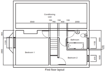
- Appendix B. Salford Energy House floor plans
- Appendix C. Salford Energy House monitoring system
- Appendix D. Flow and return temperatures
- Minutely Boiler Temperature Data - 24h NESTA - W 80°C
- Minutely Boiler Temperature Data - 24h NESTA - W 70°C
- Minutely Boiler Temperature Data - 24h NESTA - W 60°C
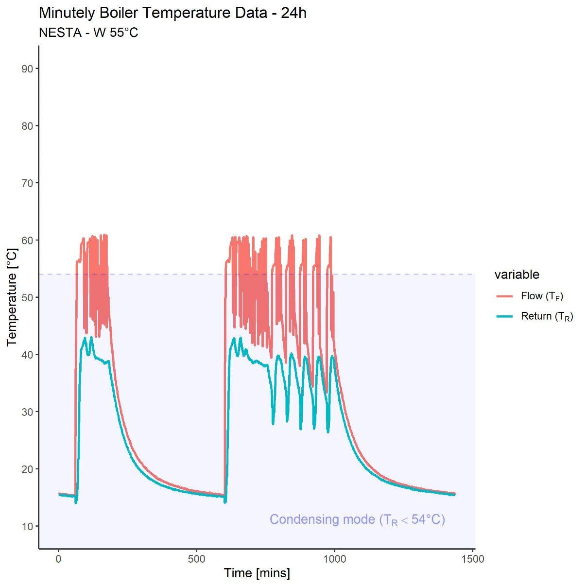
- Minutely Boiler Temperature Data - 24h NESTA - W 55°C
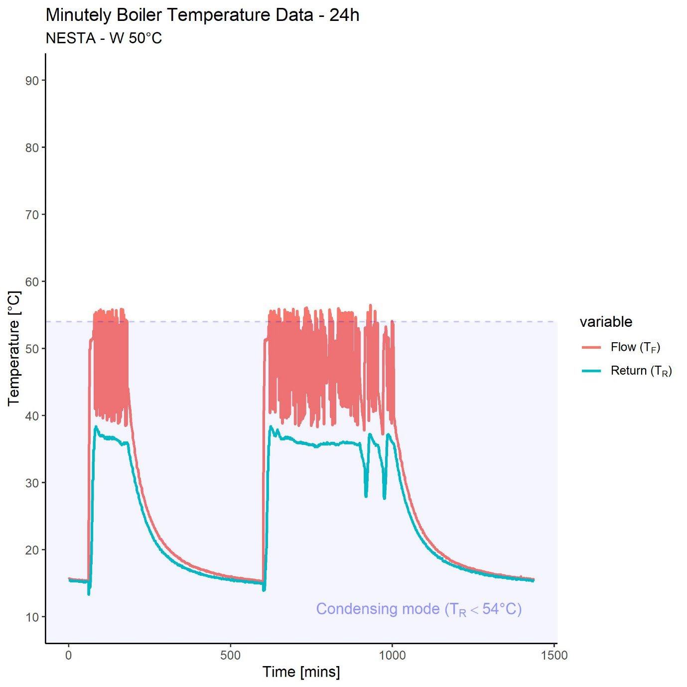
- Minutely Boiler Temperature Data - 24h NESTA - W 50°C
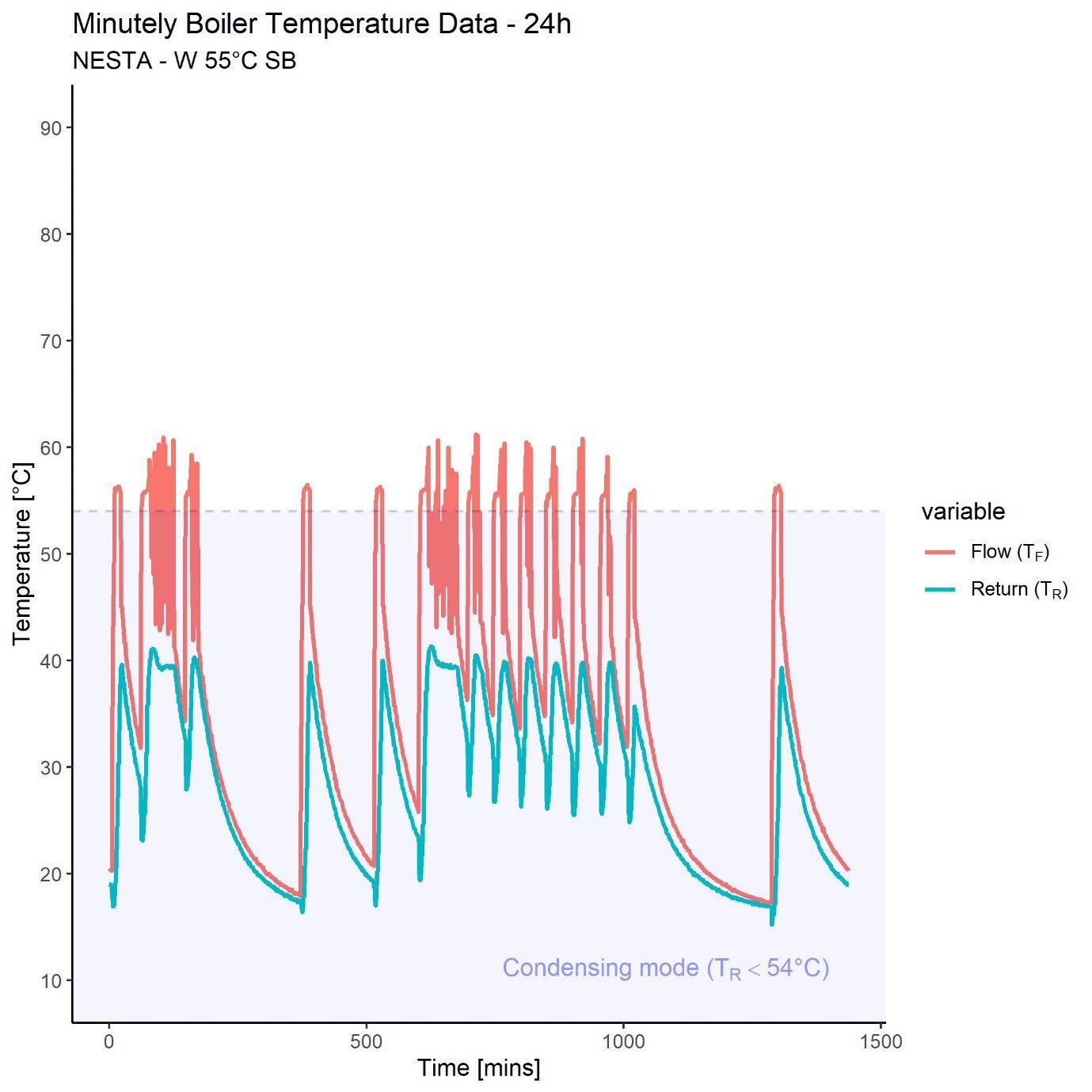
- Minutely Boiler Temperature Data - 24h NESTA - W 55°C SB
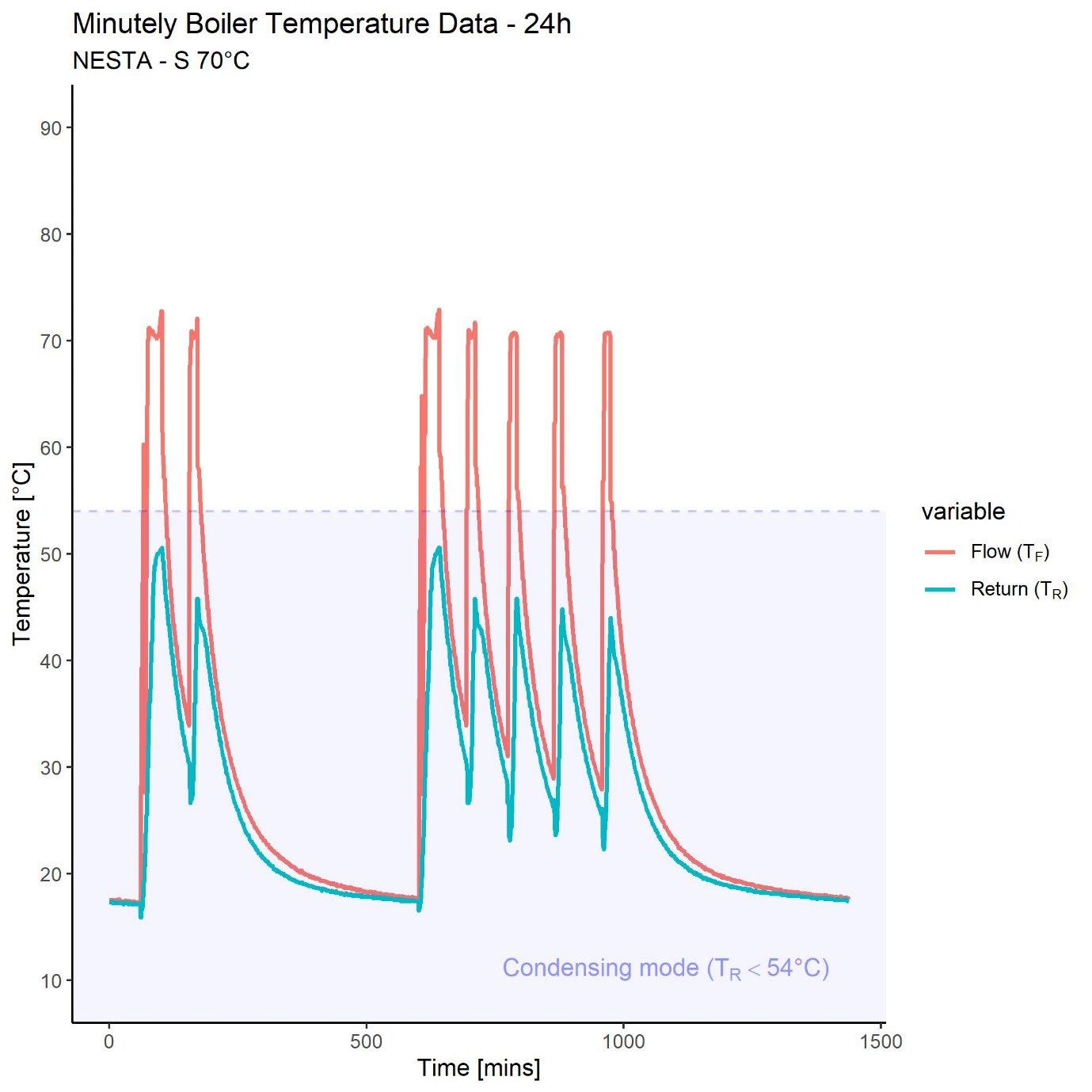
- Minutely Boiler Temperature Data - 24h NESTA - S 70°C
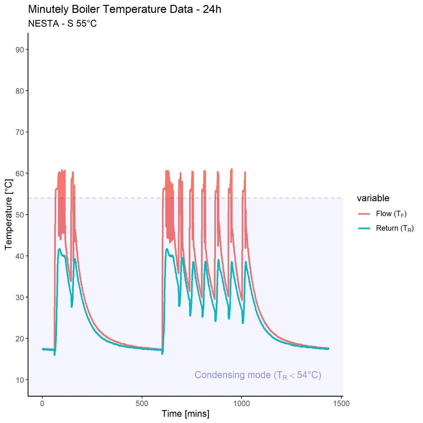
- Minutely Boiler Temperature Data - 24h NESTA - S 55°C
- Appendix E. Thermal comfort
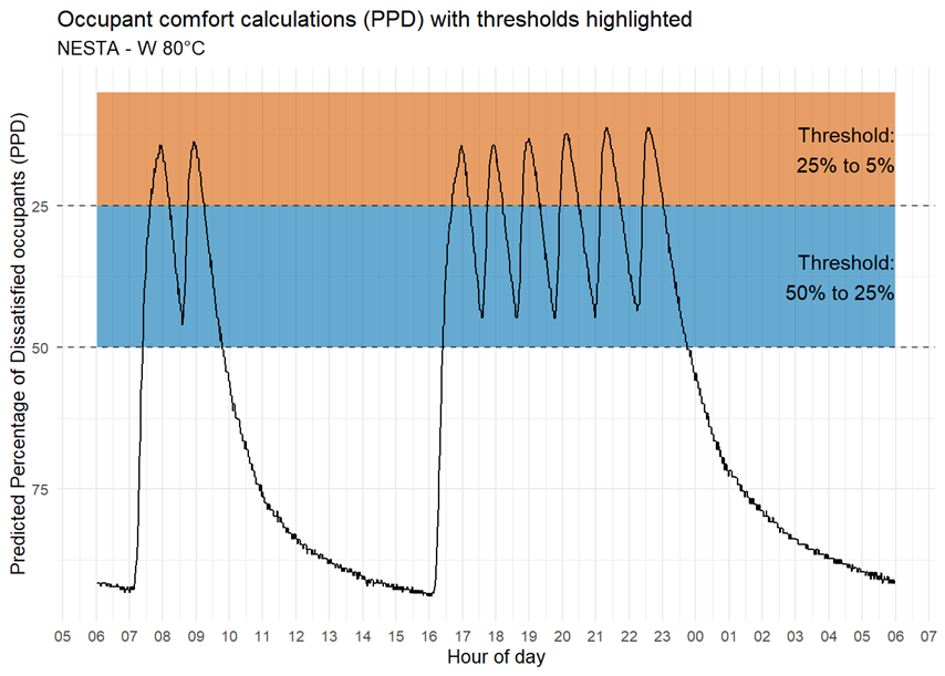
- Occupant comfort calculations (PPD) with thresholds highlighted NESTA - W 80°C
- Occupant comfort calculations (PPD) with thresholds highlighted NESTA - W 70°C
- Occupant comfort calculations (PPD) with thresholds highlighted NESTA - W 60°C
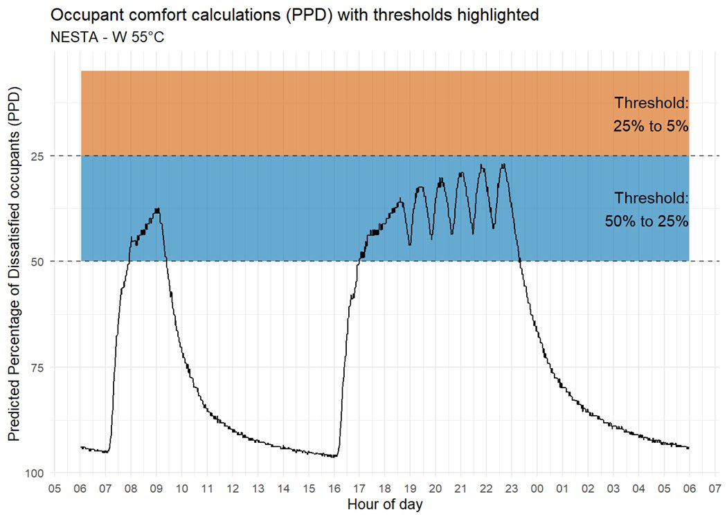
- Occupant comfort calculations (PPD) with thresholds highlighted NESTA - W 55°C
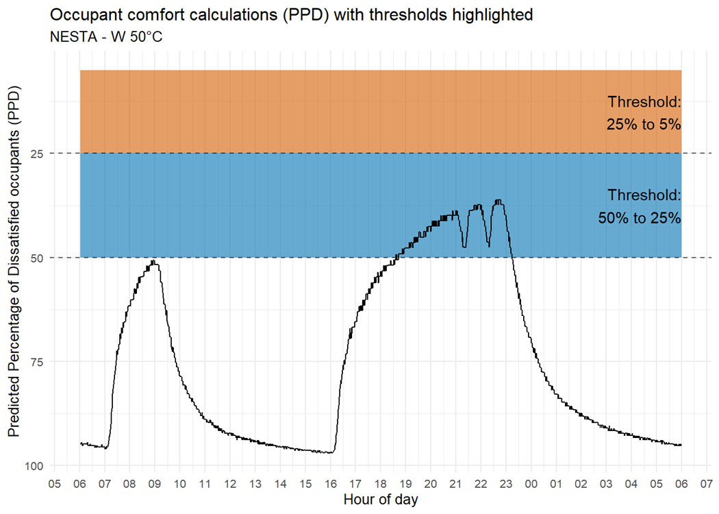
- Occupant comfort calculations (PPD) with thresholds highlighted NESTA - W 50°C
- Occupant comfort calculations (PPD) with thresholds highlighted NESTA - W 55°C SB
- Occupant comfort calculations (PPD) with thresholds highlighted NESTA - S 70°C
- Occupant comfort calculations (PPD) with thresholds highlighted NESTA - S 55°C
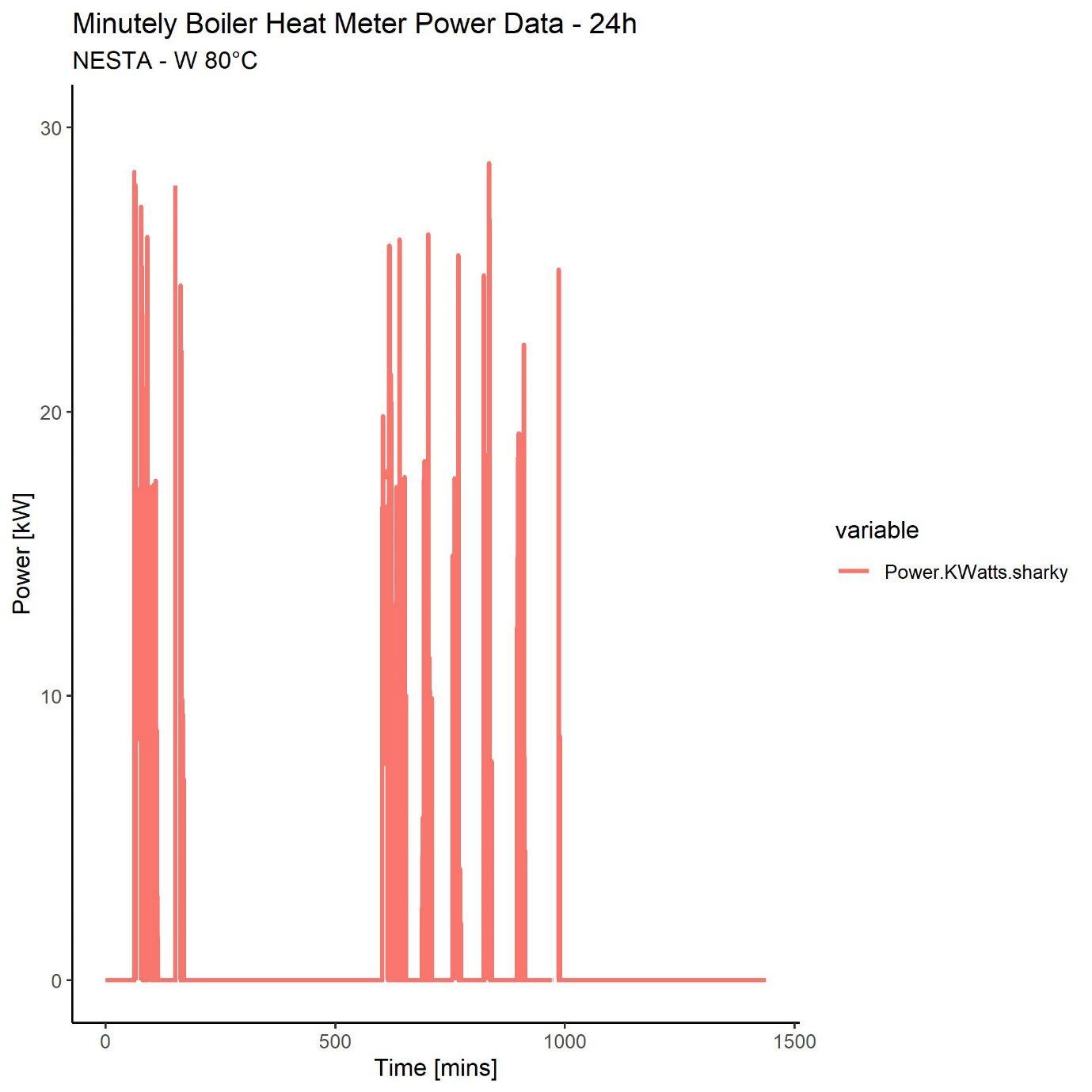
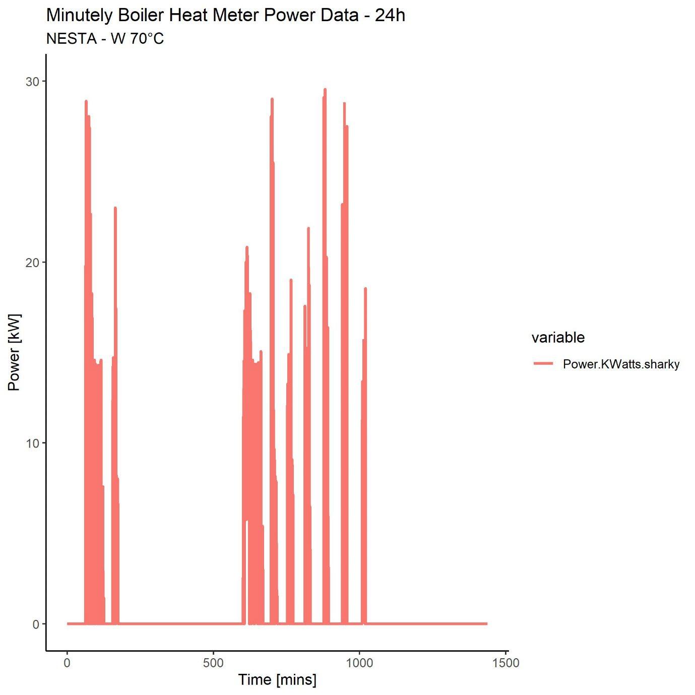
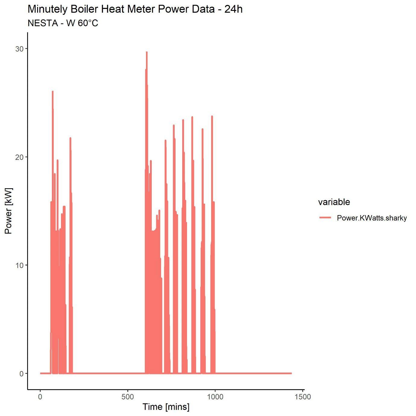
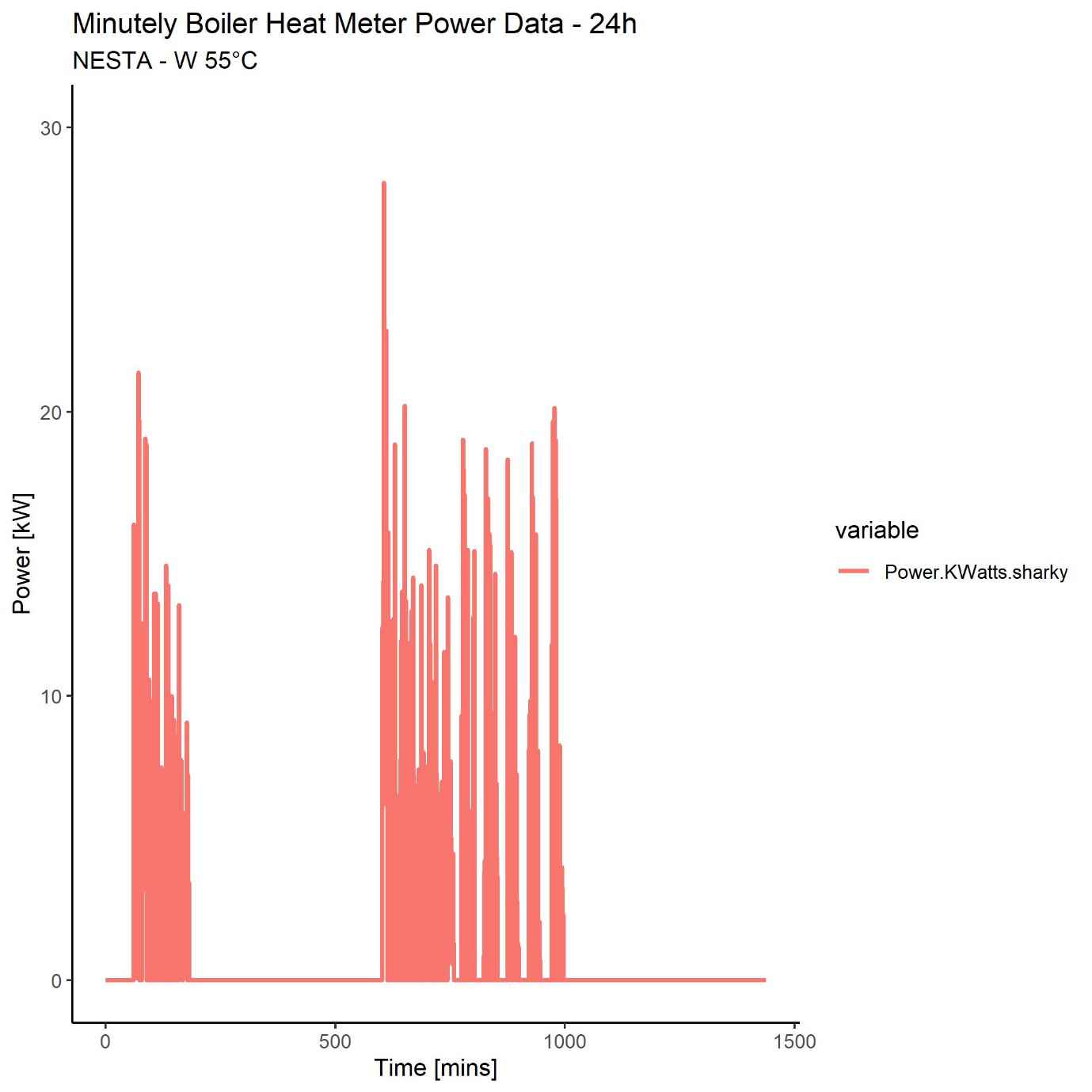
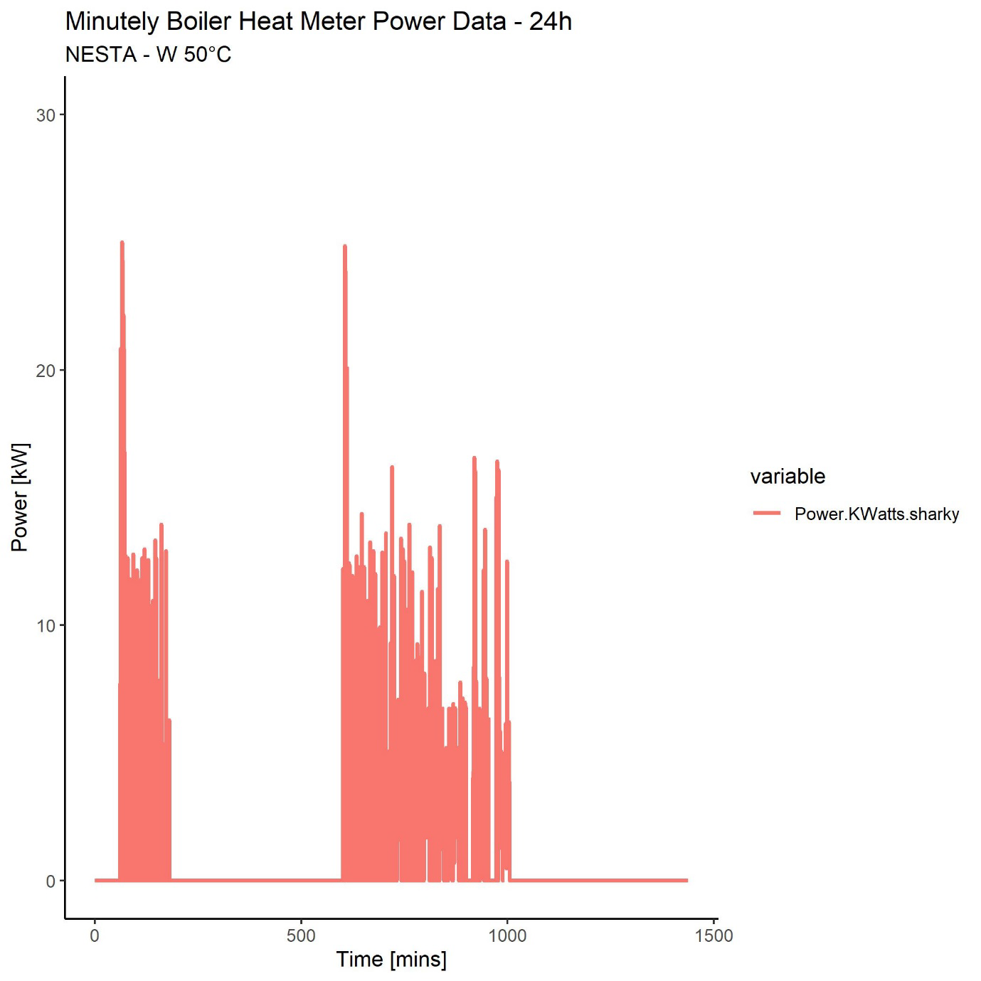
- Appendix F. Boiler power output measurements
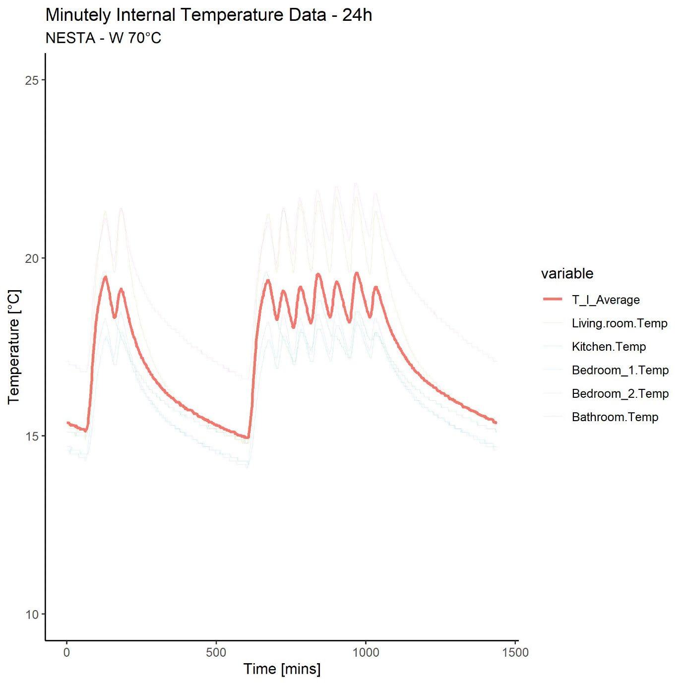
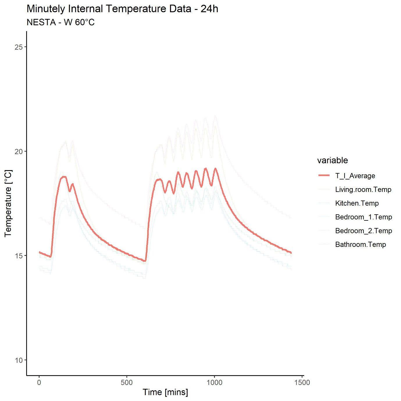
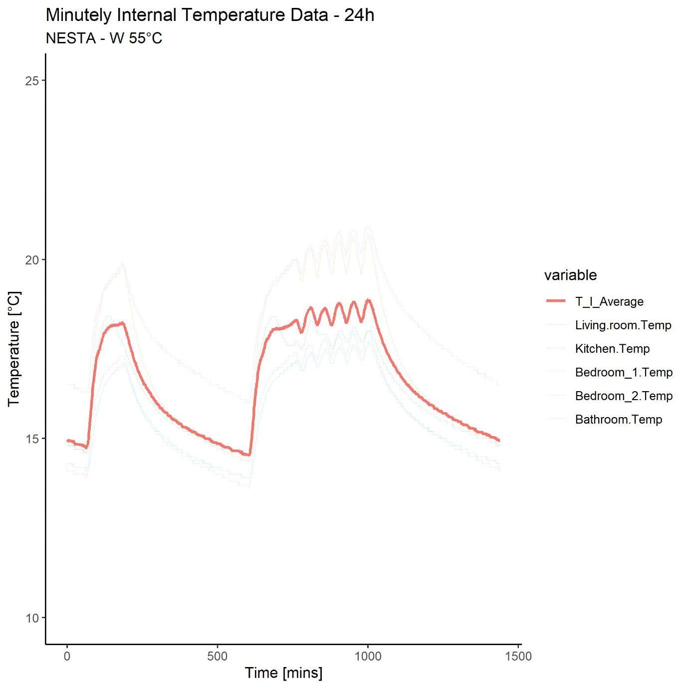
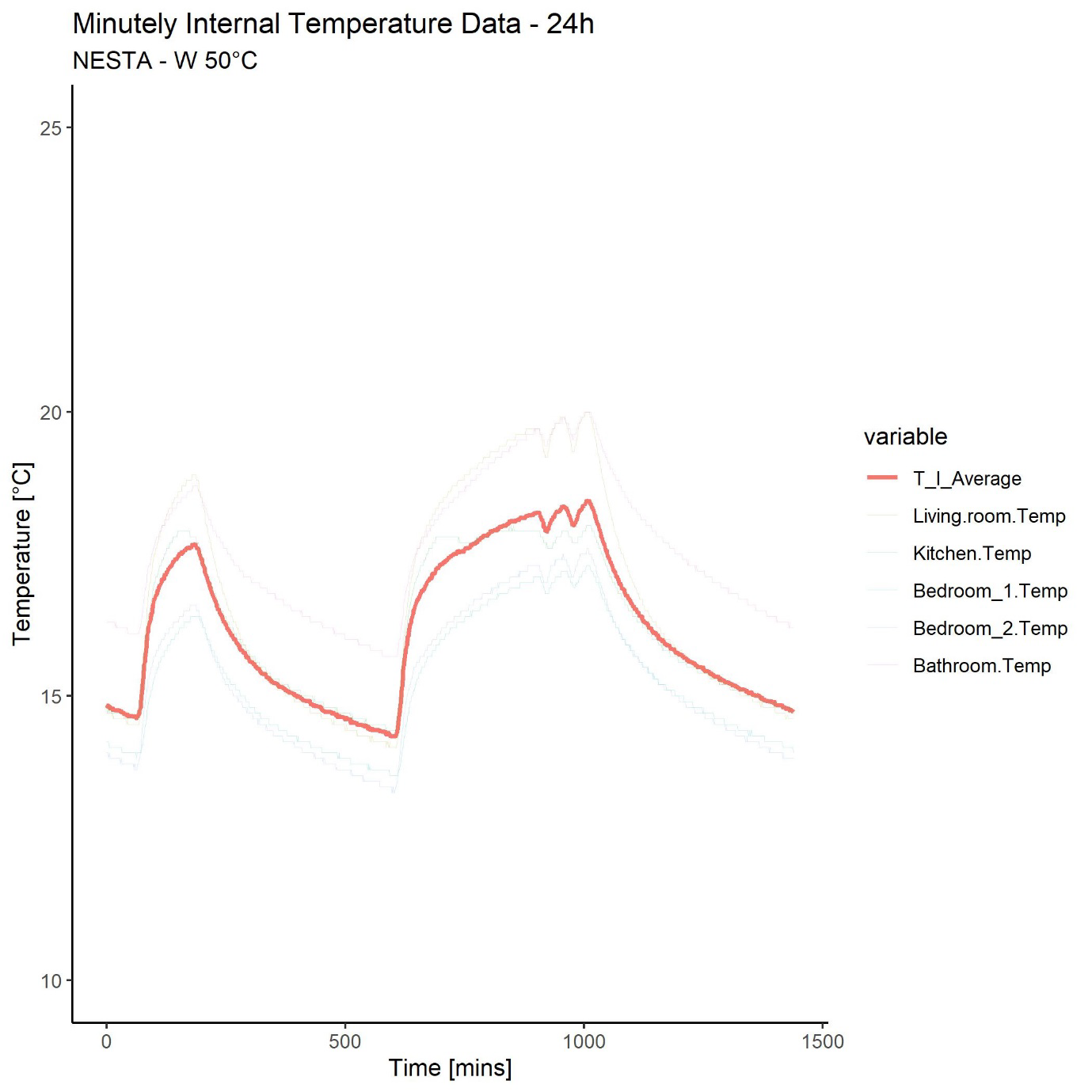
- Appendix G. Internal temperature measurements
1. Introduction
This report provides the initial results1 from the Salford Energy House Boiler Flow Temperature Testing project. It was undertaken by an Energy House Labs research team at the University of Salford (UoS) Energy House research facility and was commissioned and funded by Nesta.
Condensing boilers can recover latent heat from flue gases that would otherwise be lost to the external environment, thereby improving their efficiency. For condensing to occur, the return temperature from the central heating circuit must be below 54 °C. Condensing increases as the return temperature decreases. Lowering the flow temperature of a boiler is one way to reduce the return temperature and increase boiler efficiency. However, the impact if this intervention on space heating provision is less well understood. The purpose of this study was to investigate the impact of reducing the flow temperature of a domestic gas condensing boiler on space heating provision and energy use.
2. Methodology
2.1 Test subject
2.1.1 The Energy House
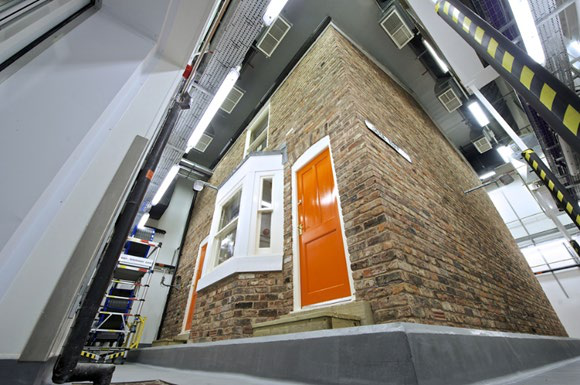
The Energy House is a replica Victorian solid wall end-terrace house constructed within an environmental chamber capable of achieving external temperatures between -12 °C to +30 °C. It was built using reclaimed materials and traditional construction methods of the time and can be retrofitted to most fabric thermal performance standards2. The hydronic central heating system of the Energy House is served by a gas boiler. The Energy House shares a party wall with a similar building, referred to as the Conditioning Void (CV). Environmental conditions in the chamber and CV can be controlled and repeated across multiple test periods. This makes it possible to measure the impact of changes to its building fabric or space heating provision with greater confidence and speed than houses in the field.
2.1.2 Energy House monitoring
The findings provided in this report are based upon the following measurements recorded at one-minute intervals by the Energy House's monitoring system3:
- gas consumption using a Siargo MF32GD10 digital gas flow meter4 (uncertainty ± 1.5-3%5)
- boiler data using a Sharkey 775 heat meter located within 500 mm of boiler connections:
- power and energy output (uncertainty ± 1%)
- flow and return temperature using PT-100 RTDs (uncertainty ± 0.3 °C)
- flow rate using an ultrasonic flow meter (uncertainty ± 1%)
- boiler electricity consumption using a Siemens 7KT PAC1200 digital power meter (uncertainty ± 2%)
- boiler OpenTherm parameters using Ovon BoilerEye
- air temperature using IC temperature sensors (uncertainty ± 0.3 °C) located at mid-storey height in the geometric centre of each room and within the environmental chamber
- black globe temperature at mid-storey height in the geometric centre of each room (uncertainty ± 0.3 °C).
2.1.3 Fabric thermal performance
The configuration of the Energy House's thermal elements for the test programme was adapted to be representative of most English solid wall dwellings, 88% of which have uninsulated external walls and 87% have full double glazing, though only 39% have 200 mm or more of loft insulation. The loft insulation depth was intended to represent homes that have been subject to low-cost fabric energy efficiency improvements through schemes such as the Energy Company Obligation (ECO). Table 2 provides the configuration and thermal performance of the Energy House's thermal elements during the test programme.
Table 2. Configuration and thermal performance of Energy House elements during test programme
| Thermal element | Construction | CIBSE DHDG | Measured |
|---|---|---|---|
| External walls | 225 mm solid wall with 12.5 mm wet plaster | 2.11 | 1.65 |
| Roof | Cold roof with 270 mm insulation at ceiling level | 0.16 | 0.14 |
| Ground floor | Suspended timber (carpeted in living room) | 0.83 (living room) | 0.81 (living room) |
| 0.90 (kitchen) | 0.88 (kitchen) | ||
| Windows | 'E' rated double glazing units in PVCu frames | 2.80 | 2.42 |
| Doors | 'E' rated PVCu doors (rear half glazed) | 1.80 | 0.99 (front) |
| 1.71 (rear) | |||
| Party wall | Solid wall with plaster finish on both sides | 1.33 | 1.40 |
Table 2 shows that most of the U-values assumed by the 2017 version of the CIBSE Domestic Heating Design Guide (DHDG) are in reasonable agreement with the measured fabric performance of the Energy House. This provides a reasonable level of confidence that the heat load of the Energy House calculated using this methodology is suitable for the purposes of the test.
Table 3 provides whole house metrics of building fabric thermal performance for the Energy House during the test programme. The SAP rating of 67 is in good agreement with the average SAP rating in England of 66. The air permeability value is comparable with UK average of 11.5 m³.h⁻¹.m² @ 50 Pa7.
Table 3. Whole house metrics of thermal performance for the Energy House during the test programme8
| Metric | Value |
|---|---|
| Heat transfer coefficient (measured) | 170 W/K |
| Heat loss parameter (measured) | 3 W/m²K |
| Air permeability (measured) | 12.7 m³.h⁻¹.m² @ 50 Pa |
| SAP rating (RdSAP) | 67 (Band D) |
| Design heat load @ -3 °C (CIBSE DHDG) | 6.6 kW |
2.1.4 Gas central heating system
The Energy House has a conventional hydronic central heating system with radiators in each room served by an Intergas Xclusive 24 kW combination boiler. The boiler is capable of a turndown ratio of 7:1, so can modulate its output between 25.1 and 3.6 kW.
The heat load and radiators were sized by an independent building services engineer using the 2017 version of the CIBSE DHDG based on a flow temperature of 70 °C and a return temperature of 50 °C. The 2017 version was used to reflect central heating installs performed before the introduction of ErP boiler control classification under the Boiler Plus legislation in 2018 that incentivised the uptake of more advanced controllers that are capable of modulating boiler output. The difference between the calculated heat load and installed heat output of the radiators was <1%. The output from the heat load and radiator sizing calculation is provided in Table 4.
Table 4. CIBSE DHDG heat load and radiator sizing calculation
| Zone | Design temp (°C) | Air change rate (ACH) | Heat load (W) | Installed capacity (W) |
|---|---|---|---|---|
| External | -3 | |||
| Living room | 21 | 1.5 | 2,086 | 2,092 |
| Kitchen | 18 | 2 | 1,577 | 1,521 |
| Stairs | 18 | 1.5 | 135 | 287 |
| Landing | 18 | 1.5 | 130 | |
| Bedroom 1 | 18 | 1 | 1,236 | 1,240 |
| Bathroom | 22 | 1.5 | 681 | 652 |
| Bedroom 2 | 18 | 1 | 768 | 733 |
| Total | 6,613 | 6,525 |
The boiler in its optimised state was considered unrepresentative of typical UK boilers. Nesta requested that its parameters be changed to replicate the behaviour of a Worcester Greenstar I Junior of the 2010-15 era. This is considered a good benchmark for the boiler setup, due to this product being one of the most common boilers fitted into UK homes and still prevalent in the UK market. The Worcester Greenstar I Junior has a minimum burner modulation of 7kW, which is also very typical of many other brands of boilers still on the market today. The Worcester Greenstar I Junior has a fixed speed pump set for speed 3 (approximately 6 meters head). This appliance has no burner anti-cycle or energy saving features, apart from domestic hot water pre-heat.
The Energy House has a calculated heat load of 6.6 kW at -3 °C external air temperature which is below the minimum boiler modulation, but this is very typical in many properties in the UK. When dealing with the heating system flow rate, the problem with replicating the pump pressure of a Worcester Greenstar I Junior is that system balancing (especially to the required heating system design of 70/50) is very difficult to achieve when balancing 'statically' (using traditional radiator lockshield valves and temperature clamps across the radiator). The heating consultant suggested that 'dynamic' balancing thermostatic radiator valves (TRVs) should be fitted, to aid the system balancing, as they maintain the correct flow rate irrespective of system pressure. The Drayton 'auto-balancing' TRV was selected to simplify installation time and reduce balancing issues associated with traditional balancing methods.
The Intergas boiler's heat exchanger was cleaned and tested for combustion performance in accordance with manufacturer's instructions. The boiler's fan speed was adjusted to achieve a minimum fan speed to replicate 7 kW minimum heat input and the boiler was set to a maximum heat input of 24 kW (to replicate a boiler that was not range rated) and this was verified using the Energy House's gas meter data. The burner anti-cycle time was set to two minutes and any such boiler energy saving features were disabled, again to replicate the poor characteristics of gas condensing boilers of the period. The heating system was tested for operation and the air was fully purged from the system, via bleeding the radiators and the boiler's primary heat exchanger bleed point. The Drayton TRV's were set to achieve the designed setpoints in each room. Drayton's online TRV calculator was used to obtain the correct flow rates for the radiator output based on the radiator size and construction, flow temperature and system temperature drop of the radiators. The flow rates given by the online calculator were verified against actual calculated flow rates and they were set on each TRV using the manufacturer's instructions. Two simulated test runs were performed which deemed the system suitable for the tests to proceed.
The controls selected for this research were a Class I Honeywell Home T6360 thermostat. This is one of the most common thermostats fitted to UK homes and is prevalent in the domestic heating market. Nesta wanted to replicate 'setback' temperatures for some of the tests, so a two-thermostat setup was prepared using a single channel timer to switch between the two products at different times. As the Intergas boiler can only accept an extra low voltage signal for heating demand, an extra low voltage switching relay was incorporated into the thermostat build for volt free switching. The anticipators on the T6360s were activated on each of the controllers and were installed at mid-room height on an internal wall in the living room (Figure 1).
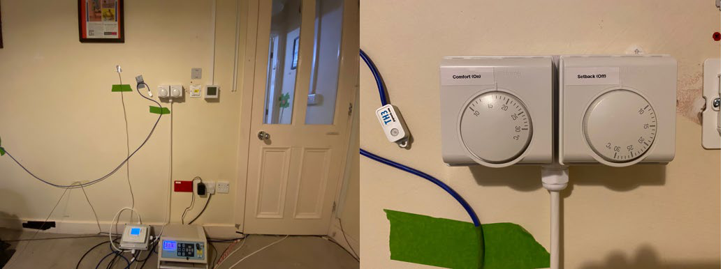
Figure 1. Thermostatic controllers on the living room wall (right thermostat provides setback control)
2.2 Test conditions
2.2.1 Internal environment
The internal set-point temperatures were based on the design temperatures using in the CIBSE DHDG calculation (Table 4). The interlock thermostat was set to maintain 21 °C in the living room, with TRVs set to maintain ~18 °C in all zones except the bathroom, which was set to 22 °C9. Prior to testing, the thermostats and TRVs were adjusted to achieve setpoint temperatures at the centre of each room at a 70 °C flow temperature.
The CV neighbouring the Energy House was maintained at 20 °C throughout the test programme.
The Energy House was heated using the SAP pattern of 07:00-09:00 and 16:00-23:00. Where setback temperatures were used between heating periods, the setback living room thermostat was set to 17 °C with no change to the TRVs.
2.2.2 External environment
Table U1 of SAP10 was used to select external temperatures considered representative of the UK average during the SAP heating season (October to May). The heating season was split into winter (December to February) and shoulder (autumn and spring) seasons to assess heating system performance during part- and full-loads. The weighted mean temperature (based on number of days in each month) during each season was used to select the chamber chiller setpoints. The chamber HVAC was set to achieve 4.2 °C during the winter test period and 8.9 °C during the spring test period.
2.3 Test programme
Table 5 provides the test programme. To minimise thermal mass effects resulting from charging and discharging of the building fabric, each test was a minimum of 72 hours in duration. The initial 48-hour period allowed the Energy House to reach a state of dynamic equilibrium. Prior testing at the Energy House has shown that 24-hour periods following the initial 48-hour stabilisation period produces repeatable results thereafter. The final 24-hour period for each test was the reporting period.
Table 5. Test sequence, identifiers, & configuration (W and S denote winter and shoulder seasons, respectively)
| Test id | W80 | W70 | W60 | W55 | W55-SB | W50 | S70 | S55 |
|---|---|---|---|---|---|---|---|---|
| Flow setpoint (°C) | 80 | 70 | 60 | 55 | 55 | 50 | 70 | 55 |
| Chamber setpoint (°C) | 4.5 | 4.5 | 4.5 | 4.5 | 4.5 | 4.5 | 9 | 9 |
| Heating pattern | SAP | SAP | SAP | SAP | SAP setback | SAP | SAP | SAP |
3. Results
3.1 Flow and return temperatures
Table 6 summarises the boiler flow and return measurements for each test. The values are based on the average flow and return temperatures across the entire heating circuit during the initial heat-up periods in each test. They provide the most reliable indication of how the system is balanced as they only consider periods when the boiler is firing and all the TRVs are open.
Table 6. Boiler flow and return temperatures during initial heat-up periods across tests
| Test id | Flow setpoint temp (°C) | Flow temp (°C) | Return temp (°C) | ΔΤ (°C) |
|---|---|---|---|---|
| W80 | 80 | 80 (± 0.3) | 55 (± 0.3) | 25 (± 0.4) |
| W70 | 70 | 70.2 (± 0.3) | 50.6 (± 0.3) | 19.6 (± 0.4) |
| W60 | 60 | 60.8 (± 0.3) | 46.3 (± 0.3) | 14.5 (± 0.4) |
| W55 | 55 | 55.1 (± 0.3) | 43 (± 0.3) | 12.1 (± 0.4) |
| W50 | 50 | 48.2 (± 0.3) | 38.4 (± 0.3) | 9.8 (± 0.4) |
| W55-SB | 55 | 55.4 (± 0.3) | 41.3 (± 0.3) | 14.1 (± 0.4) |
| S70 | 70 | 70.4 (± 0.3) | 50.6 (± 0.3) | 19.8 (± 0.4) |
| S55 | 55 | 55.7(± 0.3) | 41.7 (± 0.3) | 14 (± 0.4) |
Figure 2 shows that, at each flow temperature setting, the boiler provided reasonably accurate control of flow temperature. At the 70 °C flow temperature setting, the system was behaving close to the 70/50 °C design specification.
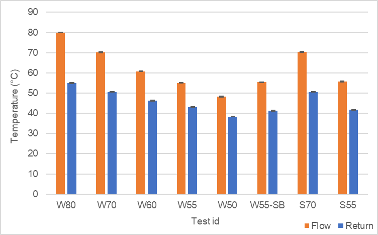
Figure 2. Average boiler flow and return temperatures during heat-up period
Figure 3 shows the temperature difference (ΔT) across the whole heating circuit during the periods used to calculate the values provided in Figure 2. It shows that the ΔT across the system is dependent on the flow temperature setting and that the system becomes more unbalanced from the design ΔT of 20 °C at 70 °C as the flow temperature is reduced. Lower ΔTs indicate a lower heat output from the radiators due to a lower mean water temperature transferring less heat into the dwelling and vice versa.
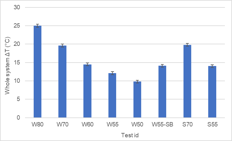
Figure 3. Whole system ΔT across tests
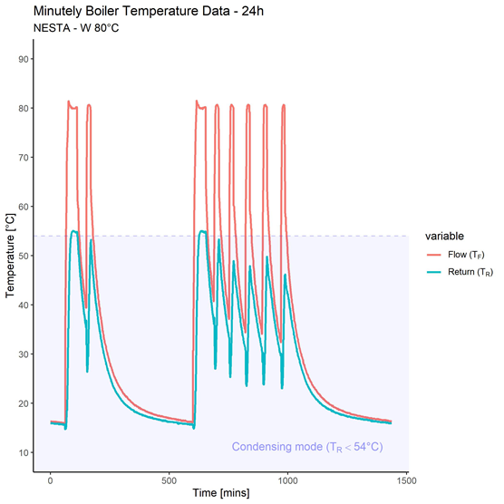
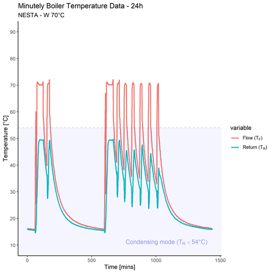
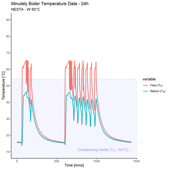
Figure 4 and Figure 5 show the flow and return temperatures measured across the entire 24-hour reporting period of each winter test (larger versions of these graphs can be found in Appendix D). At 80 °C (W80), the boiler spends a large proportion of its time in condensing mode while firing. This is due to the ΔT at 80 °C being greater than the design ΔT of 20 °C. Reducing the flow temperature below 80 °C resulted in the boiler being permanently in condensing mode while firing. As the flow temperature is reduced, the return temperature also reduces, thereby increasing the condensing capability and efficiency of the boiler.
During the 55 °C (W55) and 50 °C (W50) flow tests, the flow temperatures measured when the boiler was firing were below the temperature required for condensing to occur, especially at 50 °C flow temperature. This maximised the surface area of the heat exchanger where condensing could occur, resulting in the greatest levels of efficiency measured during the test programme.
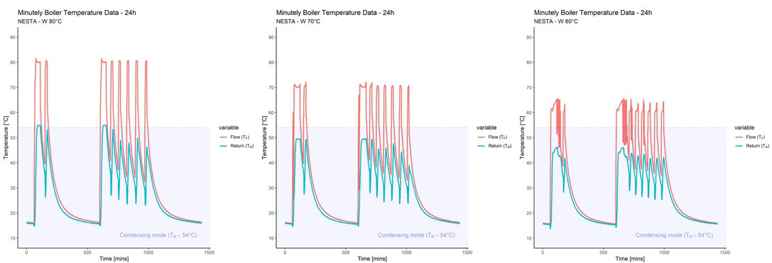
Figure 4. 24h flow and return temperatures for the W80, W70 and W60 tests
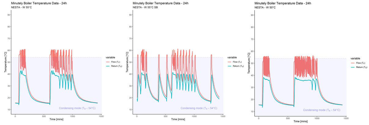
Figure 5. 24h flow and return temperatures for the W55, W55-SB and W50 tests
3.2 Internal air temperature
Table 7 summarises the 24-hour volume weighted average internal air temperatures during each test.
Table 7. 24-hour volume weighted average internal air temperatures
| Test id | 24h mean external temp (°C) | 24h average internal temp (°C) | ΔΤ (°C) | Min average temp (°C) | Max average temp (°C) | ΔΤ change on 70°C baseline |
|---|---|---|---|---|---|---|
| W80 | 4.5 (± 0.5) | 17.3 (± 0.6) | 12.8 (± 0.8) | 15.1 (± 0.6) | 20.2 (± 0.6) | +2% |
| W70 | 4.5 (± 0.5) | 17.1 (± 0.6) | 12.6 (± 0.8) | 14.9 (± 0.6) | 19.6 (± 0.6) | |
| W60 | 4.5 (± 0.5) | 16.8 (± 0.6) | 12.3 (± 0.8) | 14.7 (± 0.6) | 19.2 (± 0.6) | -2% |
| W55 | 4.6 (± 0.5) | 16.6 (± 0.6) | 12.0 (± 0.8) | 14.5 (± 0.6) | 18.9 (± 0.6) | -5% |
| W50 | 4.6 (± 0.5) | 16.2 (± 0.6) | 11.6 (± 0.8) | 14.3 (± 0.6) | 18.4 (± 0.6) | -8% |
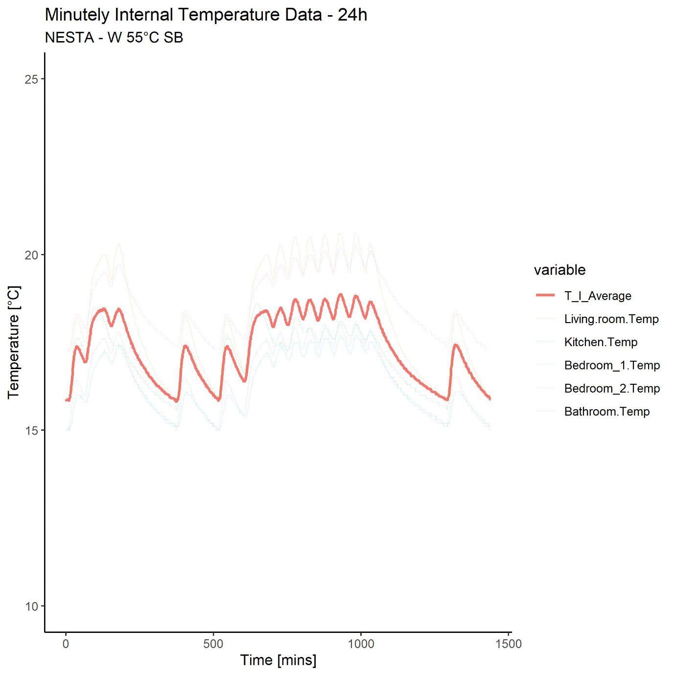
| W55-SB | 4.6 (± 0.5) | 17.3 (± 0.6) | 12.7 (± 0.8) | 15.8 (± 0.6) | 18.9 (± 0.6) | 1% |
| S70 | 9.3 (± 0.5) | 18.2 (± 0.6) | 8.9 (± 0.8) | 16.8 (± 0.6) | 20.2 (± 0.6) | |
| S55 | 9.3 (± 0.5) | 18.0 (± 0.6) | 8.7 (± 0.8) | 16.8 (± 0.6) | 19.3 (± 0.6) | -2% |
Figure 6 provides box plots summarising the volume weighted average internal air temperatures throughout each test.
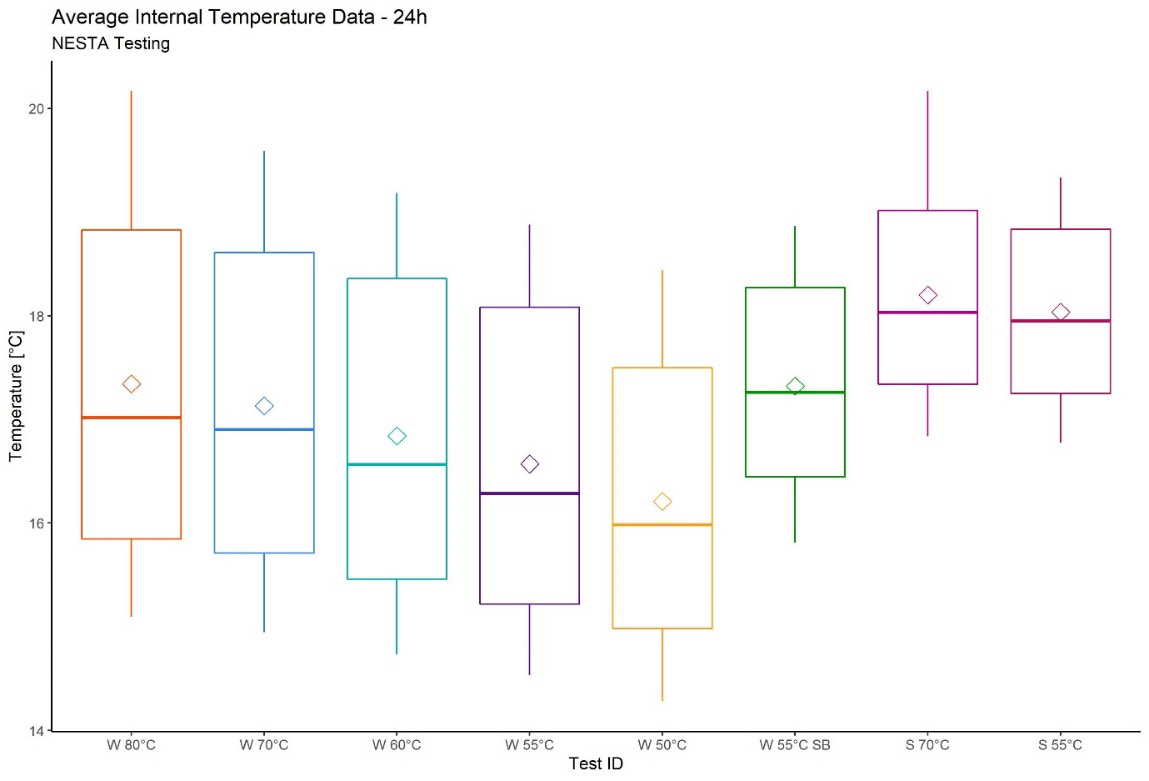
Figure 6. Box plots summarising the volume weighted average internal air temperatures
Except for the 55 °C with setback test (W55-SB), each reduction in flow temperature resulted in a reduction in internal temperatures throughout the Energy House in both the winter and shoulder season scenarios. The relationship between flow temperature and average internal temperature during the winter tests was nonlinear, with each reduction in flow temperature increasing the magnitude of the internal temperature reduction. The impact of flow temperature reduction on average internal temperature was most prominent below 60 °C (W60) in the winter scenario.
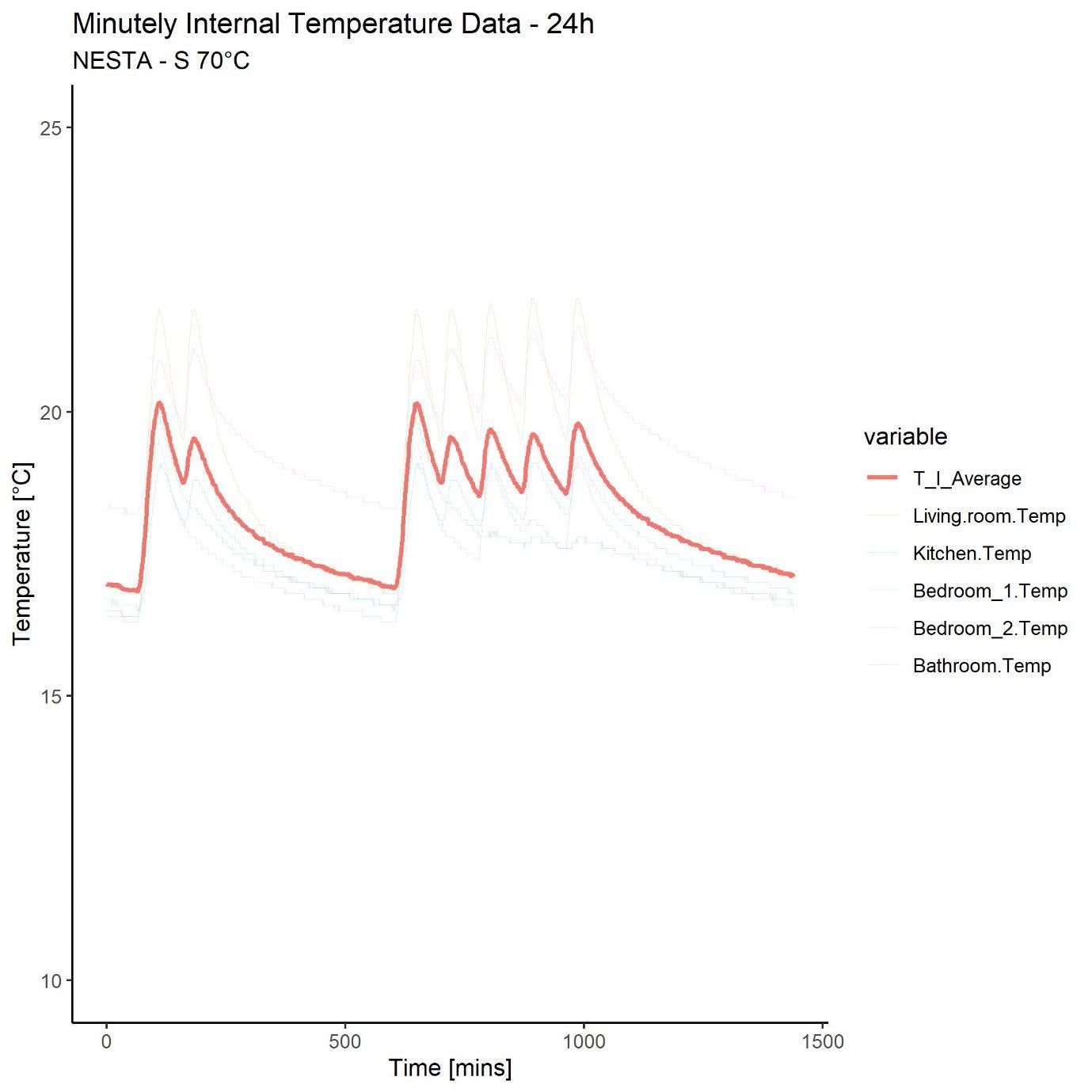
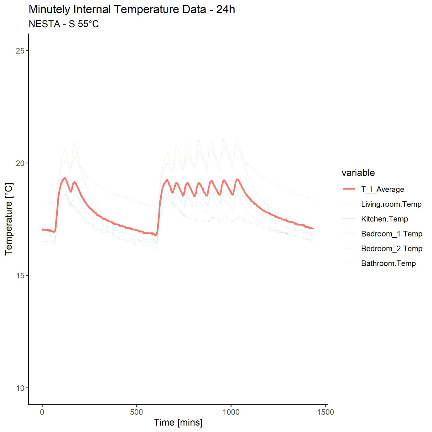
Internal temperatures during the shoulder season tests (S70 and S55) were warmer than the corresponding winter tests (W70 and W55). This can be explained by the warmer external temperature slowing the internal temperature decay between heating periods. The minimum average internal temperatures during the shoulder season tests were ~2 °C warmer than the corresponding winter tests. This also contributed to the internal environment achieving cycling temperature sooner during the shoulder season tests.
The reduction to 55 °C flow setpoint (W55) during the winter scenario resulted in an internal to external ΔT reduction of 5% from the 70 °C baseline (W70). However, the reduction from 70 °C to 55 °C during the shoulder season scenario (S70 and S55) only resulted in a 2% ΔT reduction. This indicates that a 55 °C flow setpoint is more suited to the heat demand of the Energy House during the shoulder seasons than during winter. Two percent ΔT reductions were measured in the S55 and W60 tests, meaning that the 15 °C flow setpoint reduction during the shoulder season test (S55) carried a similar ΔT reduction penalty as the 10 °C reduction during winter test (W60). This suggests that greater reductions in flow temperature are possible during the shoulder seasons than during winter, though any reduction in flow temperature will result in a reduction in internal air temperature.
Table 8 summarises the air temperature measurements for the living room and bedroom 1 during the morning (07:00-09:00) and evening (16:00-23:00) heating periods. Living room cycle temperatures and hysteresis are based on the period between the first and final full cycle during the evening heating periods.
Table 8. Air temperature measurements for the living room and bedroom 1 during the morning (07:00-09:00) and evening (16:00-23:00) heating periods
| Test id | LR median temp (°C) AM | LR median temp (°C) PM | Bed1 median temp (°C) AM | Bed1 median temp (°C) PM | LR time to cycle (mins) AM | LR time to cycle (mins) PM | LR cycle temp (°C) | Hysteresis (± °C) |
|---|---|---|---|---|---|---|---|---|
| W80 | 20.5 | 20.9 | 17.4 | 17.8 | 58 | 59 | 21.0 | 1.3 |
| W70 | 20.1 | 20.5 | 17.1 | 17.5 | 69 | 73 | 20.7 | 1.0 |
| W60 | 19.6 | 20.2 | 16.9 | 17.3 | 89 | 92 | 20.3 | 0.7 |
| W55 | 19.1 | 19.8 | 16.4 | 17.1 | - | 156 | 20.0 | 0.5 |
| W50 | 18.0 | 19.3 | 15.7 | 16.7 | - | 292 | 19.6 | 0.4 |
| W55-SB | 19.6 | 19.9 | 17 | 17.3 | 69 | 79 | 20 (SB 17.1) | 0.6 (SB 1.2) |
| S70 | 20.3 | 20.7 | 18.3 | 18.5 | 51 | 50 | 20.8 | 1.2 |
| S55 | 20.1 | 20.2 | 18.3 | 18.4 | 60 | 62 | 20.4 | 0.7 |
Figure 7 illustrates the living room internal temperature measurements during each winter test.
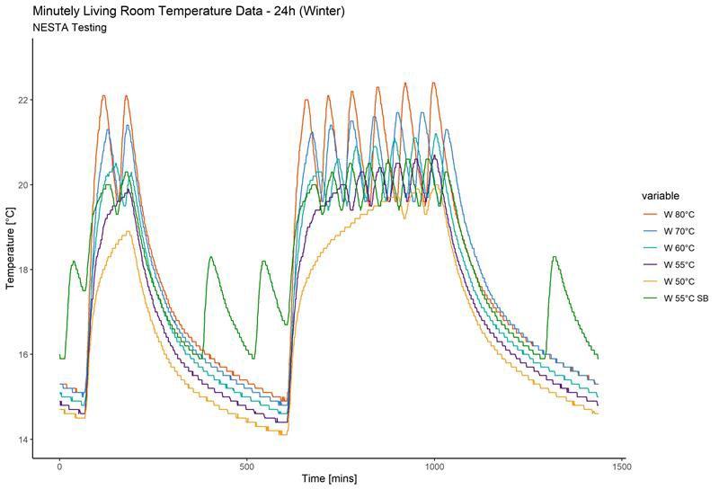
Figure 7. 24h living room internal temperature plot during all winter tests
Figure 8 illustrates the living room internal temperature measurements during the 70 °C (S70) and 55 °C (S55) shoulder season tests.
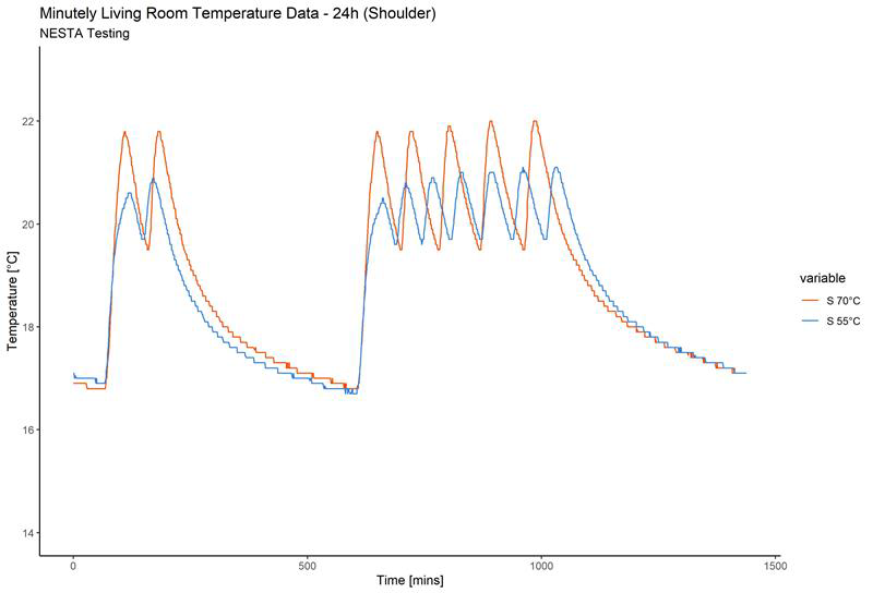
Figure 8. Living room internal temperature measurements during the shoulder season tests
Figure 9 illustrates the living room temperature during the two-hour morning heating period across all tests
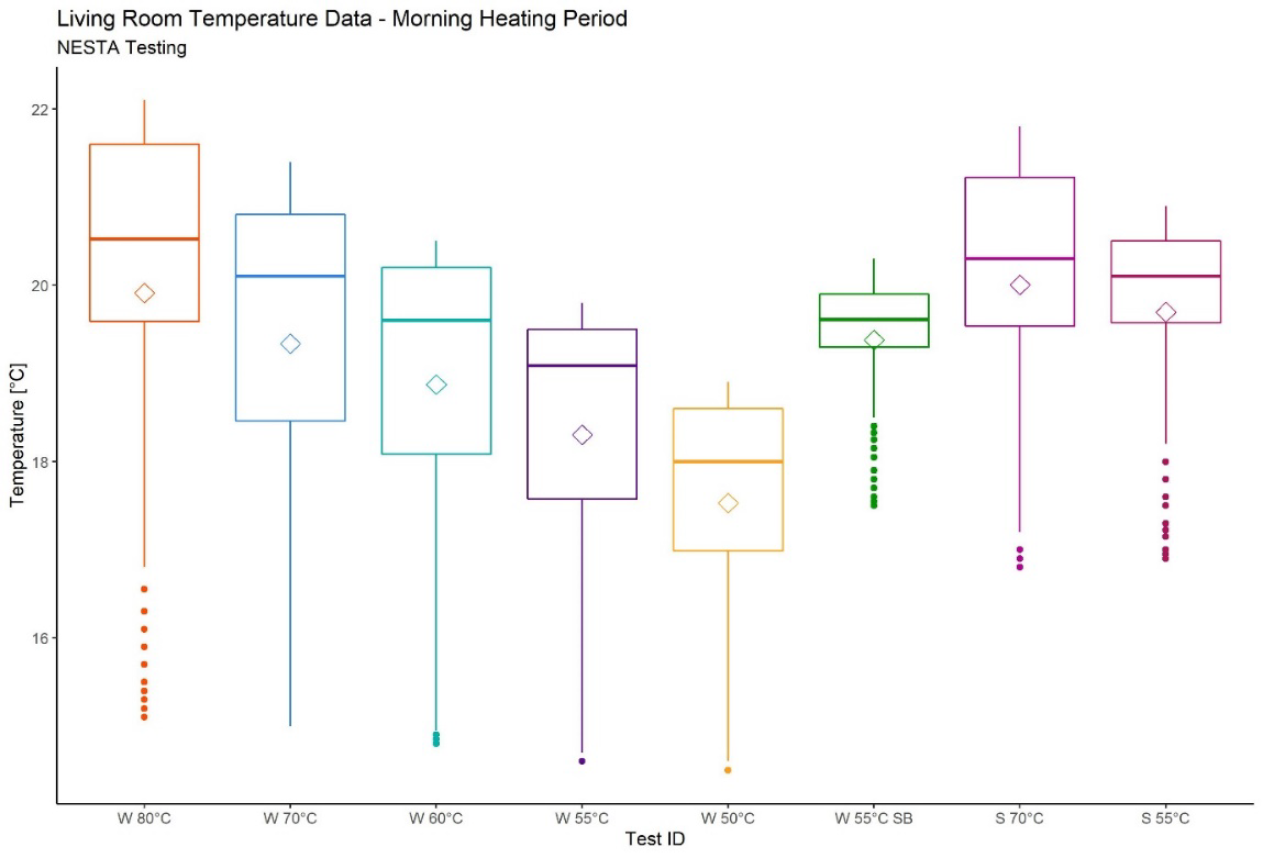
Figure 9. Box plot of living room temperature during the two-hour morning heating period across all tests
Figure 10 illustrates the living room temperature during the seven-hour evening heating period across all tests
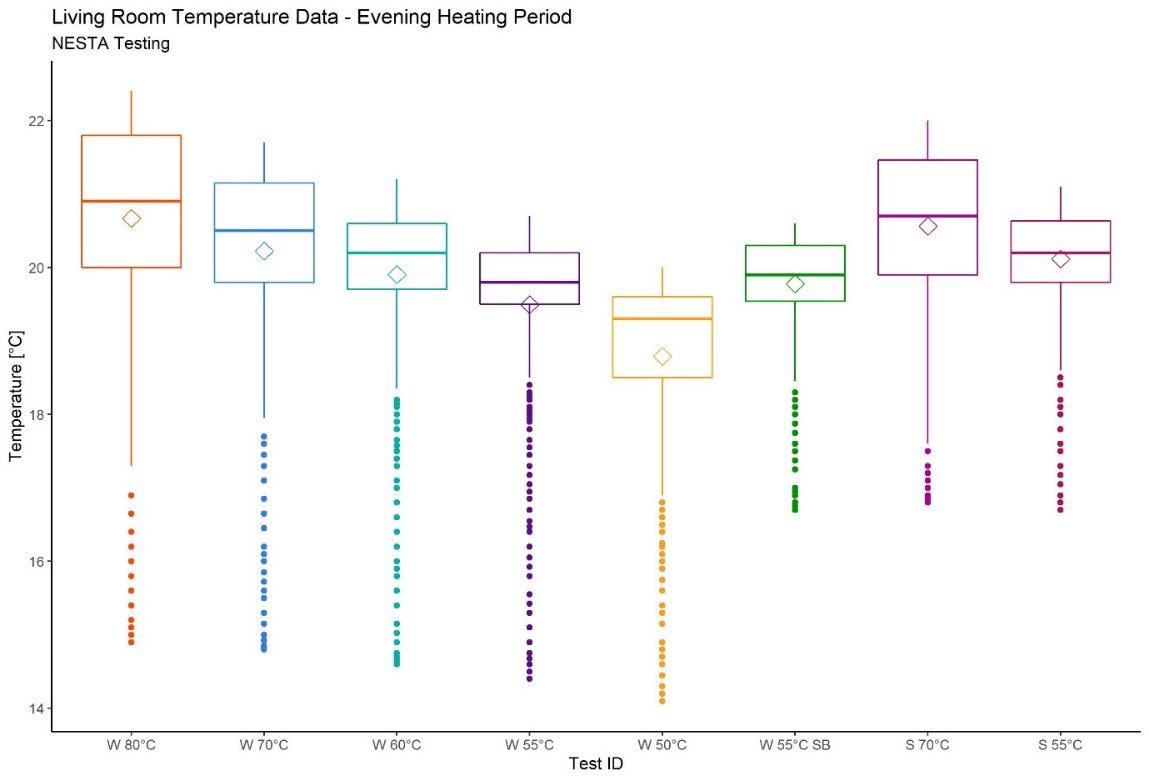
Figure 10. Box plot of living room temperature during the seven-hour evening heating period across all tests
Flow temperature reductions had a disproportionate impact on the living room internal temperature in comparison to other zones during heating periods. The living room temperature is controlled by the interlock thermostat, whereas the temperature in other zones is controlled by TRVs. The thermostat contains an anticipator designed to reduce overshooting above the setpoint. It achieves this by accounting for the residual heat output at typical flow temperatures from the interlock radiator (ie living room), and switching off the boiler before set-point is achieved. The thermostat used in this study, which is representative of basic domestic on/off Class I controls, had a fixed anticipator and could not be adjusted.
Lowering the flow temperature reduced radiator temperatures, which resulted in less residual heat output from radiators after the boiler had ceased firing. At flow temperatures below the design temperature of 70 °C, the anticipator prematurely curtailed each heating cycle before there was enough heat within the interlock radiator to enable cycling around setpoint temperature. This resulted in a reduction in the mean and maximum living room cycling temperature. The effect became more pronounced as flow temperature reduced. The minimum living room cycling temperature in each winter test was similar for all flow setpoints except 50 °C. This suggests that the 50 °C flow setpoints was insufficient to satisfy the heat demand at a 4.5 °C external temperature. TRVs do not contain anticipators, but the anticipator in the interlock thermostat influenced internal temperatures in other zones by curtailing boiler firing periods, thus preventing TRVs from cycling around setpoints.
Reducing flow temperature, and therefore the power output of radiators, slowed heat-up rates. The boiler did not cycle below a 60 °C flow setpoint during the morning heating period in the winter tests. The living room reached a maximum temperature of 18.9 °C and 19.9 °C by the end of the 55 °C (W55) and 50 °C (W50) flow setpoint tests, respectively. The failure to reach cycling temperature was due to insufficient heat input rather than anticipator behaviour. The time to reach boiler cycling (indicating thermostatic control) during the evening heating period in the winter tests substantially increased at flow temperature setpoints below 60 °C.
Reducing the flow setpoint to 55 °C (S55) during the shoulder season tests did not prevent the boiler from cycling during either the morning or evening heating period. The reduction from the 70 °C baseline (S70) resulted in a delay to boiler cycling of ~10 minutes for both heating periods. The cycling temperature reduction penalty resulting from a 15 °C reduction in flow setpoint was less severe in the shoulder season test (S55) than the winter test (W55). This indicates that a reduction to a 55 °C flow setpoint was more suited to the heat demand during the shoulder seasons test than the winter season test.
The measured internal temperature reductions were the result of lower radiator heat output increasing the time to reach cycling temperature and the behaviour of the anticipator within the thermostatic controller reducing cycling temperatures.
Introducing a setback (W55-SB) improved heat-up times and increased temperatures during both heating periods in comparison with the SAP only test (W55). The greatest benefit was during the morning where the setback resulted in cycling being achieved. Though heat-up times will be influenced by hysteresis during the set-back period as the start of peak heating periods could occur with internal temperature 1.2 °C above or below the 17 °C setback. The doubling of the hysteresis value (± 1.2 °C) at the setback temperature (± 0.6 °C during heating periods) is due to the rapid heat up rate at cooler air temperatures (which was observed across all tests). This results in the anticipator behaving in a similar manner to what was observed in the baseline tests (W70).
3.3 Thermal comfort
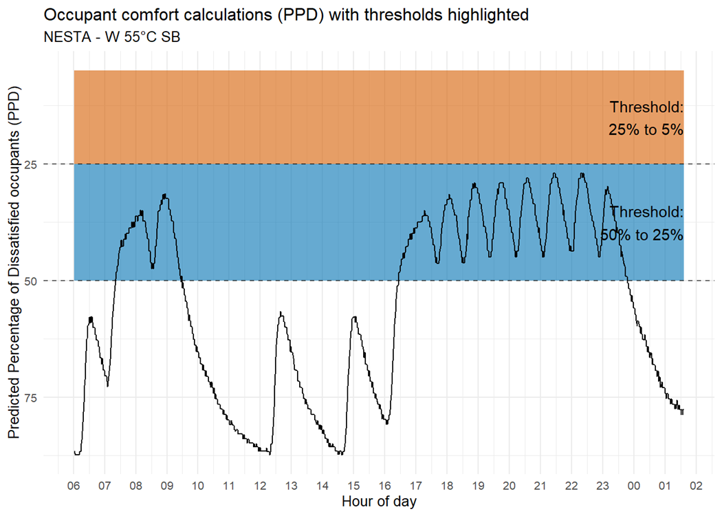
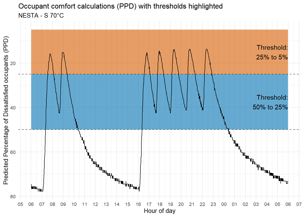
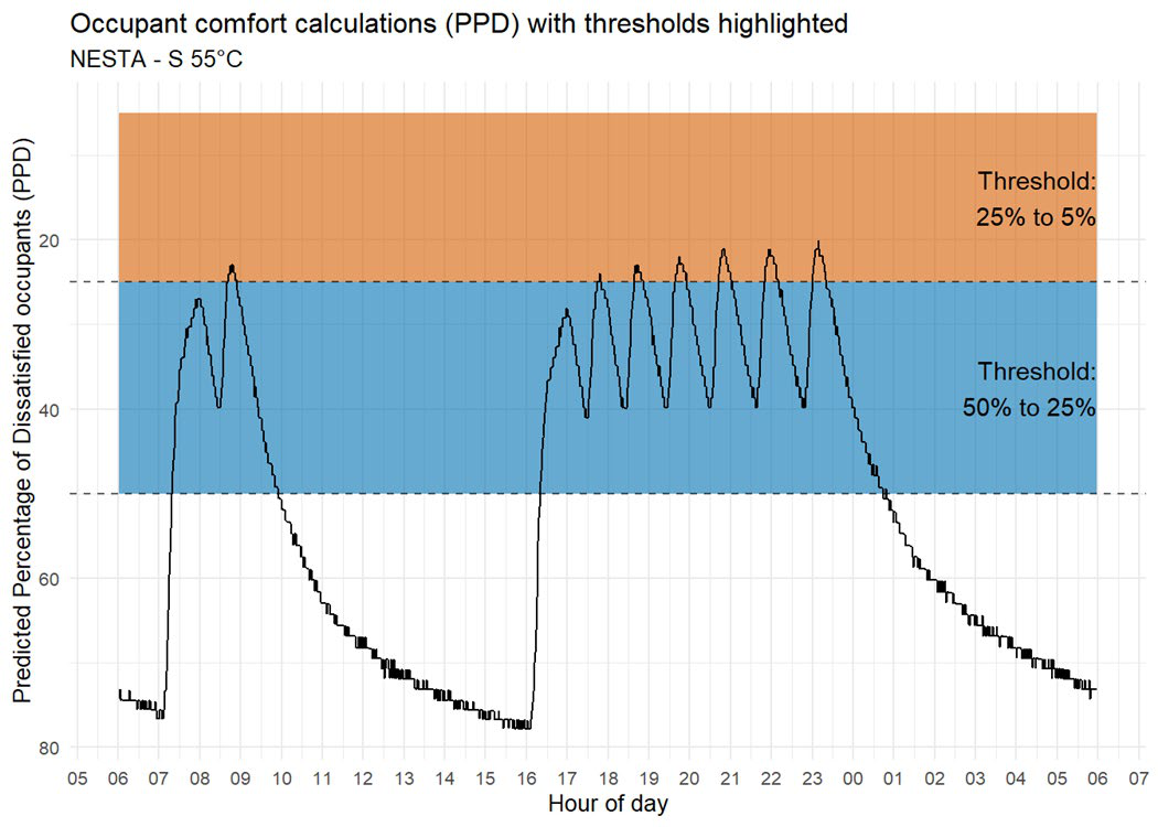
The thermal comfort of the living room was calculated using the predicted percentage of dissatisfied (PPD) index prescribed by the comfort standards ASHRAE 55 and ISO 7730. The PPD gives the estimated percentage of people who would be dissatisfied by the current thermal conditions; a lower PPD indicates a higher proportion of people are comfortable. The graphs in Figure 11 and Figure 12 have the PPD on the Y axis (has been reversed); a more favourable, lower PPD score is presented as further along the y axis than a less favourable, higher PPD score. In essence, a PPD score of 50% calculates that half of the theoretical occupants would be satisfied with the conditions in the space. A PPD score of 25% calculates that 75% of theoretical occupants would be satisfied with the conditions in the space. It must be noted that thermal comfort calculations are not applicable to all humans as the model contain multiple assumptions, so should be treated with caution. Please refer to Appendix E for details of the thermal comfort calculation method.
Table 9 summarises the findings from the thermal comfort calculations for the morning and evening heating period in each test.
Table 9. Proportions of morning and evening heating periods at varying thermal comfort thresholds for each test
| Test id | Time to < 50% PPD (mins) | Proportion of AM heating period spent in each threshold | Proportion of PM heating period spent in each threshold |
|---|---|---|---|
| AM | PM | > 50% PPD | |
| W80 | 23 | 24 | 19% |
| W70 | 30 | 31 | 25% |
| W60 | 37 | 41 | 31% |
| W55 | 56 | 59 | 47% |
| W50 | - | 157 | 100% |
| W55-SB | 20 | 26 | 17% |
| S70 | 22 | 20 | 18% |
| S55 | 20 | 21 | 16% |
Figure 11 and Figure 12 show PPD in the living room over 24-hour periods in the winter 70 °C (W70) and 60 °C (W60) flow setpoint tests, respectively. Graphs for all test periods can be found in Appendix E.
Occupant comfort calculations (PPD) with thresholds highlighted NESTA - W 70°C
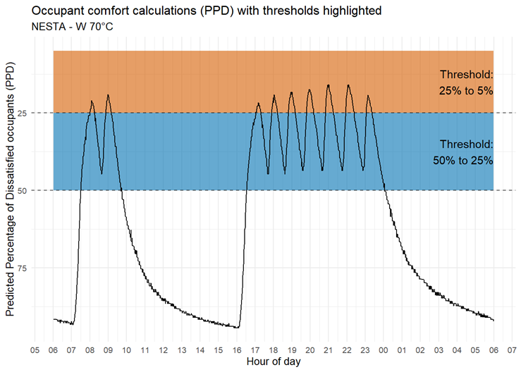 Figure 11. 24h time series of the PPD within the living room during the winter 70 °C flow temperature test
Occupant comfort calculations (PPD) with thresholds highlighted NESTA - W 60°C
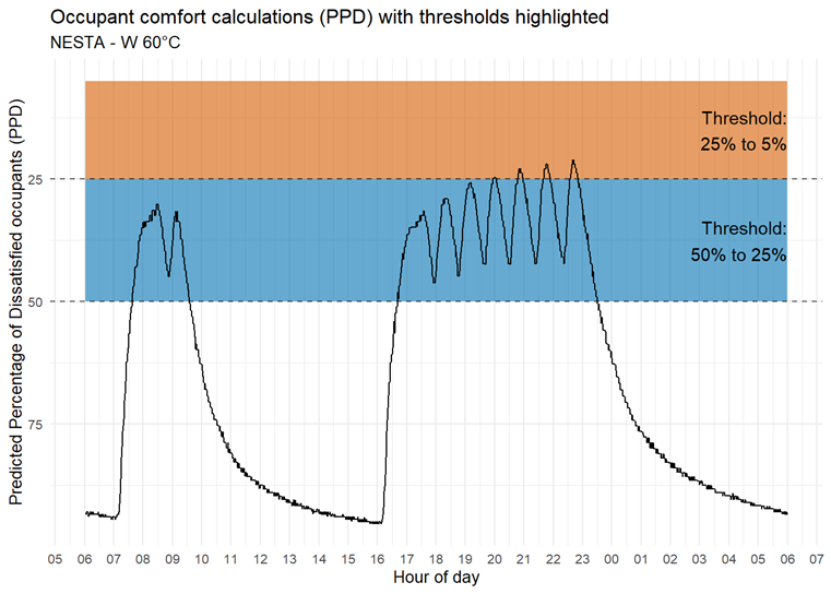 Figure 12. 24h time series of the PPD within the living room during the winter 60 °C flow temperature test
Figure 13 and Figure 14 illustrate the proportion of time spent within each PPD threshold during the morning and evening heating periods, respectively.
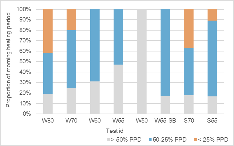 Figure 13. Plot showing PPD within the living room during the two-hour morning heating period across all tests
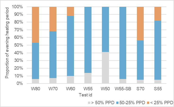 Figure 14. Plot showing PPD within the living room during the seven-hour evening heating period across all tests
Thermal comfort calculations show that occupant satisfaction with the internal environment decreases as flow setpoint is reduced due to the reduction in internal temperature. The PPD values at 70 °C flow setpoint during winter (W70) are predominately within the 50% to 25% thresholds. As this test was used as a baseline, it was decided that < 50% PPD should be the threshold that constitutes occupant satisfaction with the internal environment. Because cycling temperatures were found to vary across each test, the < 50% PPD was used as the benchmark to assess heat-up times.
The greatest detriment to occupant satisfaction during the winter tests occurred after the flow setpoint was reduced below 60 °C. It resulted in substantial increases in the time taken to reach < 50% PPD. At 55 °C flow setpoint (W55), almost half the morning heating period was spent below the < 50% PPD threshold. A 50 °C flow setpoint (W50) resulted in the entirety of the morning heating period spent below the < 50% PPD threshold.
The use of a setback at 55 °C flow setpoint (W55) resulted in the fastest time to reach the < 50% PPD threshold during the winter tests. The duration with < 50% PPD was comparable with the 70 °C winter baseline test (W70).
The reduction to a 55 °C flow setpoint during the shoulder seasons test (S55) showed no detriment to the time taken to reach, and duration spent within, the <50% PPD threshold in comparison to the 70°C baseline (S70). This indicates that occupants will be more comfortable with lower flow temperature setpoints during the shoulder seasons.
3.4 Boiler efficiency
Table 10 summarises the boiler10 and system11 efficiency measurements for each test. Change in boiler efficiency from 70 °C and 80 °C flow temperature baselines are illustrated in Figure 15.
Table 10. Boiler and system efficiencies, electrical energy consumption, boiler firing time and percentage point change on baseline for all tests
| Test id. | Boiler efficiency (%) | System efficiency (%) | Boiler electric (kWh) | Boiler firing time (mins) | Change in boiler efficiency (percentage points) |
|---|---|---|---|---|---|
| 70 °C baseline | |||||
| W80 | 83 (± 2.5) | 83 (± 2.5) | 0.15 (± 0.003) | 218 | -1 |
| W70 | 84 (± 2.5) | 84 (± 2.5) | 0.17 (± 0.003) | 266 | |
| W60 | 88 (± 2.5) | 88 (± 2.5) | 0.2 (± 0.004) | 331 | +4 |
| W55 | 89 (± 2.5) | 89 (± 2.5) | 0.24 (± 0.005) | 419 | +5 |
| W50 | 89 (± 2.5) | 89 (± 2.5) | 0.27 (± 0.005) | 496 | +5 |
| W55-SB | 86 (± 2.5) | 86 (± 2.5) | 0.23 (± 0.005) | 400 | +2 |
| S70 | 87 (± 2.5) | 86 (± 2.5) | 0.11 (± 0.002) | 169 | |
| S55 | 90 (± 2.5) | 89 (± 2.5) | 0.14 (± 0.003) | 241 | +3 |
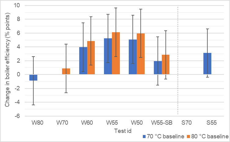 Figure 15. Change in boiler efficiency against seasonal baseline measurement
Each reduction in boiler flow temperature resulted in a further improvement in boiler efficiency from the 70 °C (W70) and 80 °C (W80) baselines across the winter tests, until reaching a maximum winter boiler efficiency of 89% at 55 °C flow setpoint (W55). The efficiency improvement from the 80 °C flow setpoint baseline was one percentage point greater at each flow setpoint than from a 70 °C baseline. A flow temperature setpoint of 80 °C reduced boiler efficiency by one percentage point compared with the 70 °C design setpoint.
Reducing the flow setpoint from 70 °C to 60 °C (W60) during the winter tests resulted in the greatest improvement in boiler efficiency (+4%) per 10 °C increment.
The use of a setback at 55 °C flow setpoint (W55-SB) reduced boiler efficiency by three percentage points on the SAP only 55 °C winter test (W55). The reason for this is unclear as boiler efficiency during the SAP and setback periods were similar.
Due to the boiler operating at part-load during the shoulder seasons tests (S70 and S55), boiler efficiency was greater than the corresponding winter tests (W70 and W55). The greatest boiler efficiency measured during the test programme was 90% during the shoulder seasons 55 °C flow temperature test. The 70 °C baseline boiler efficiency during the shoulder seasons test (87%) was three percentage points greater than the 70 °C winter test (84%). The relatively high baseline during the shoulder seasons test explains why the improvement in efficiency on a 70 °C baseline at 55 °C was lower for the shoulder test (+3%) than the winter test (+5%).
Figure 16 shows the relationship between return temperature and boiler efficiency for the winter and shoulder seasons SAP tests.
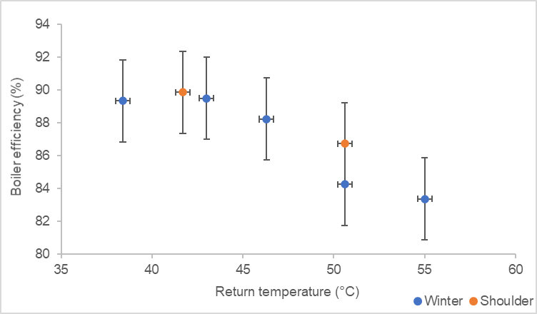 Figure 16. Scatter plot showing how boiler efficiency varies with boiler return temperature
Boiler efficiency improved as return temperature decreased in the winter tests until plateauing at 89%. This relationship was expected due to increased heat recovery of flue gasses. However, efficiency should have improved further at 50 °C flow setpoint with a return temperature of 38.4 °C. Rapid on/off boiler behaviour at 50 °C flow setpoint is thought to be the reason for no increase in efficiency at this stage (refer to Section 3.5 / Figure 19).
Figure 17 shows the relationship between boiler firing duration and boiler electricity consumption.
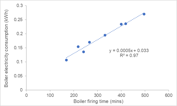 Figure 17. Scatter plot showing how boiler electricity consumption linearly increases with boiler firing time
There is a very strong relationship between boiler firing time and boiler electricity consumption. Increased electrical energy consumption is related to the operation of the pump (intercept suggests 14 W consumption when not firing). The close agreement between boiler and system efficiency (Table 10) shows that the pump operation had little impact on system efficiency. The test boiler was modern and has an efficient pump. Longer operation of an older and less efficient pump may have a greater impact on system efficiency.
3.5 Gas use
Table 11 summarises the gas use and boiler output for each test.
Table 11. Gas use and boiler output for each test
| Test id | Gas use (kWh) | Boiler output (kWh) | Change in gas use |
|---|---|---|---|
| 70 °C baseline | |||
| W80 | 47.8 (± 1.2) | 39.9 (± 0.4) | 5% |
| W70 | 45.4 (± 1.1) | 38.2 (± 0.4) | |
| W60 | 42 (± 1.1) | 37.1 (± 0.4) | -7% |
| W55 | 40.1 (± 1.0) | 35.9 (± 0.4) | -12% |
| W50 | 36.8 (± 0.9) | 32.8 (± 0.3) | -19% |
| W55-SB | 45.7 (± 1.1) | 39.4 (± 0.4) | 1% |
| S70 | 27.8 (± 0.7) | 24.1 (± 0.2) | |
| S55 | 24.3 (± 0.6) | 21.8 (± 0.2) | -13% |
Change in gas use from seasonal 70 °C and 80 °C flow setpoint baselines are illustrated in Figure 18.
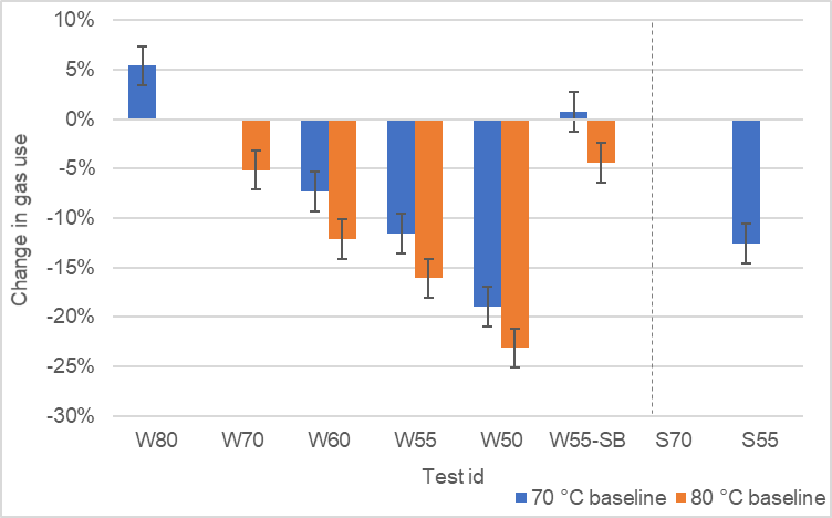 Figure 18. Change in boiler gas consumption against seasonal baseline measurement
Each reduction in boiler flow temperature resulted in a further reduction in gas use from the 70 °C (W70) and 80 °C (W80) baselines across the winter tests. The reduction in gas use from a 80 °C flow setpoint baseline was approximately four percentage points greater at each flow setpoint than from a 70 °C baseline. A flow setpoint of 80 °C resulted in a 5% increase in gas use compared with the 70 °C flow design setpoint. A 15 °C reduction in flow setpoint during the shoulder seasons tests (S70 to S55) reduced gas use by one percentage point more than when compared to the winter tests (W70 to W55).
The use of a 17 °C setback at a 55 °C flow setpoint (W55-SB) increased gas use by 1% on the 70 °C baseline (W70) and by 14% on the 55 °C SAP only heating pattern (W55). The higher average internal temperatures and reduced boiler efficiency during the setback test could explain the increases in gas use.
Figure 19 illustrates the gas flow rates at 10 °C increments during the evening heating period of the winter tests.
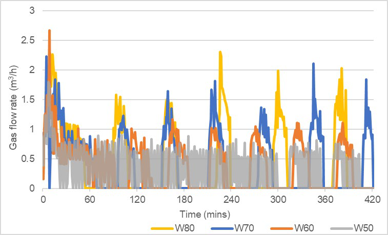 Figure 19. Gas flow rate behaviour across 10 °C increments during the 7h evening heating period of the winter tests
Figure 19 shows that although the boiler fires for a greater duration at lower flow temperatures, the rate of gas consumption during firing periods is also reduced. Rapid on/off boiler behaviour was evident when boiler flow temperature drops below 55 °C, indicating that required heat output is below the minimum capability of the boiler. The rapid on/off behaviour at the 50 °C flow temperature could explain why no efficiency improvement was measured below 55 °C. The reduction in the rate of gas consumption at lower flow temperatures partially explains why increased boiler firing time does not result in a total increase in gas consumption (the other reason being the increased boiler efficiency).
The percentage change in volume weighted average internal-external ∆T is a reasonable approximator for the change in heat demand. Figure 20 shows the relationship between change in 24-hour average internal-external ∆T and 24-hour gas use from the 70 °C baseline in the winter tests (W70).
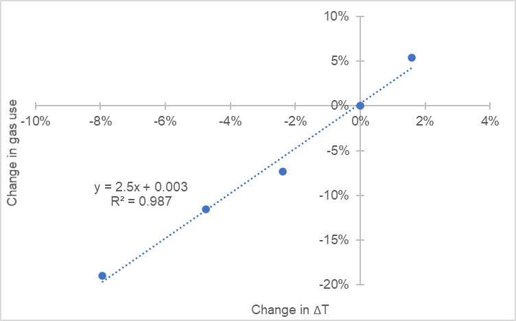 Figure 20. 24-hour average internal-external ∆T vs 24-hour gas use from the 70 °C baseline in the winter tests (W70)
There is a very strong relationship between change in ∆T and change in gas use from the 70 °C baseline (W70). However, reductions in gas use were 2.5 times greater than the reduction in ∆T (analogous to heat demand). This suggests that reductions in heat demand are not the main reason for the measured reductions in gas use. Therefore, the measured reductions in gas use are primarily attributed to improvements in boiler efficiency.
4 Conclusions and recommendations
The tests found that reducing the flow temperature of a condensing gas boiler reduces space heating gas use. This is primarily attributed to increased boiler efficiency resulting from a lower boiler return temperature. However, reducing the boiler flow temperature also reduces radiator heat output which results in slower heat-up rates and lower internal temperatures during heating periods. The research team cannot recommend an ideal boiler flow temperature reduction as this will depend upon individual thermal comfort requirements.
It is inevitable that lower radiator temperatures will result in more time being required to achieve setpoint temperatures. Lowering the flow temperature too far can result in setpoint not being achieved, especially for short heating periods, or heat-up times that may not be acceptable to occupants.
In theory, once system design setpoints are achieved, it should be possible to maintain setpoints using a lower flow temperature at any external temperature above the design temperature (-3 °C for the Energy House), so long as the system heat output is greater than the heat load at that temperature. However, in practice, the behaviour of a thermostat anticipator can result in a reduction in the average cycling temperature. The impact of increasing the thermostat setpoint to compensate for anticipator behaviour was not tested and could prove counterproductive.
Lower flow temperatures reduce cycling temperature hysteresis and setpoint overshoot. Provided the heat load is satisfied, the minimum temperature experienced while cycling is reasonably consistent across all flow temperatures. A more consistent internal temperature may provide a thermal comfort benefit that mitigates the reduction in average cycling temperature. Further research into the effects of hysteresis on thermal comfort is required.
Reducing flow temperature during the shoulder seasons (spring and autumn) has less impact on internal conditions than a similar reduction during winter. Therefore, the shoulder seasons offer the greatest potential for space heating gas use savings by reducing flow temperature. Greater understanding of the impact of the boiler flow temperature on internal conditions may allow occupants to optimise the efficiency of their boiler by varying the boiler flow temperature to suit external conditions throughout the heating season.
Setting the flow temperature above the design temperature causes a boiler to be less efficient, which results in increased gas use. Those that currently have a flow temperature setpoint greater than the design flow temperature have the greatest potential for gas use savings from a reduction in flow temperature. However, they will also notice the greatest change in heat-up times and internal temperatures.
Use of a setback temperature between heating periods results in increased gas consumption. This suggests that it is more cost effective to switch heating off between heating periods for dwellings like the Energy House. However, using a lower flow temperature with setback may provide a cost-effective way for households to avoid large temperature fluctuations between peak heating periods (eg home workers, intermittent daytime occupancy).
As reducing boiler flow temperature reduces internal temperature and slows heat-up rates, it may not be advisable to recommend this energy saving strategy alongside a reduction in thermostat setpoint temperature. Reducing thermostat setpoint may be a more suitable energy saving strategy for households that require space heating for shorter periods of time as it will have less impact on heat-up times. However, households that require longer heating periods may gain greater benefit from reducing boiler flow temperature due to an improvement in boiler efficiency. Either strategy will mean occupants facing a trade-off between their competing desires for thermal comfort and lower heating bills.
The study did not consider some issues that may influence the potential gas savings that could result from a reduction in boiler flow temperature:
- Fabric thermal performance. The fabric thermal performance characteristics of a dwelling will influence its space heating energy requirement and occupant's thermal comfort. These characteristics include the U-values and thermal mass of elements and airtightness. The percentage savings in gas use measured may be considered reasonably representative of this archetype but may differ for others within the UK housing stock. Findings from this study are being used to inform modelling to predict gas savings across other archetypes.
- External conditions. The study did not consider external temperatures below 4.5 °C. Theoretically, internal design temperatures cannot be achieved if the flow temperature is reduced when the external temperature is at or below the external design temperature (-3 °C for the Energy House). It is also important that occupants following a flow temperature reduction strategy know how to increase the flow temperature if required.
- Occupant behaviour. Occupant behaviour was not included in this study. Some occupants may not accept the reduced internal temperatures, increased heat-up times, or cooler radiators, resulting from lower flow temperatures. Others may respond by making other changes to the heating system that could influence space heating gas use (eg increasing thermostat set-points or heating periods).
- Self-learning thermostats. The study considered a basic Class I on/off thermostatic controller. Some thermostatic controllers use learning algorithms to predict heat-up times. This is used to ensure set-point is reached at the commencement of a heating period by pre-heating the dwelling. Increased heat-up times could result in controllers commencing heating earlier. This could compensate for the reduction in thermal comfort at the commencement of each heating period, but it could reduce the potential for energy savings. At very low flow temperatures, it is possible that pre-heating may commence so early that gas use is increased. Individual heating control manufacturers may need to provide guidance on this matter.
Complementary technologies
Boiler controllers with weather compensation dynamically adjust the flow temperature depending on the external air temperature. Findings from this study compliment a previous study which suggests that controls with weather compensation could provide significant gas savings 12, so their adoption for existing systems should be encouraged. However, many existing boilers are not compatible with such controls, or they could be unaffordable to householders.
Remote OpenTherm monitoring could provide stakeholders (eg householders, social housing providers) with information about the performance of their boilers that could assist with optimisation. The OpenTherm monitor installed at the Energy House provides a web-based method of viewing boiler parameters (Figure 21). Although primarily used for fault detection, such devices could be used to identify boilers with flow temperatures set above design values or poorly balanced systems that require balancing.
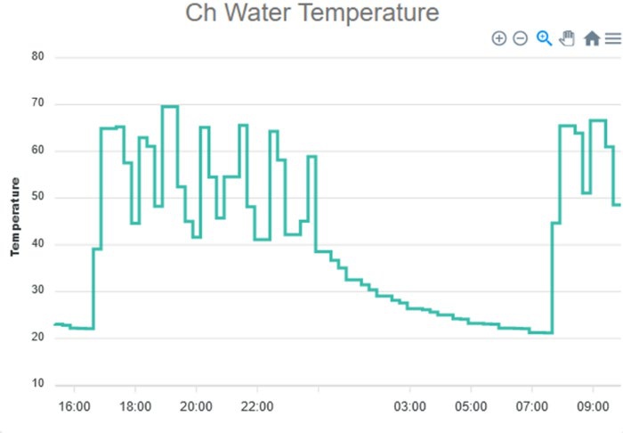 Figure 21. Example of the web-based OpenTherm monitoring of boiler parameters
Appendix A. Salford Energy House construction details
Table A1. Salford Energy House construction details
| Thermal element | Construction |
|---|---|
| External walls | Solid wall - 222.5 mm brick arranged in English bond (5 courses) with 9 mm lime mortar and 10.5 mm British Gypsum Thistle hardwall plaster with a 2 mm Thistle Multi-Finish final coat. The ground and intermediate floor joists are built-in to the gable wall. |
| Roof | Purlin and rafter cold roof structure with 270 mm insulation at ceiling level. 100 mm mineral wool insulation (λ 0.044 W/mK) between 100x50 mm ceiling joists. 170 mm mineral wool (λ 0.044 W/mK) above and perpendicular to joists. Ceiling joists run parallel to the gable wall at 400 mm centres above lath (6 mm) and plaster (17 mm) ceiling |
| Ground floor | Suspended timber ground floor above a ventilated underfloor void (20 mm depth). 150x22 mm floorboards fixed to 200x50 mm floor joists at 400 mm centres. Floor joists run between the gable and party wall with joists ends built into masonry walls. |
| Windows | 'E' rated double glazing units in PVCu frames. |
| Doors | Front - 'E' rated PVCu Rear - 'E' rated half glazed PVCu. |
| Party wall | Solid wall as external walls but with plaster finish on both sides. |
Appendix B. Salford Energy House floor plans
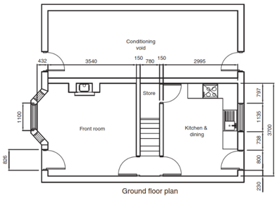
Appendix C. Salford Energy House monitoring system
The Energy House test facility is equipped with a monitoring system that records a comprehensive array of parameters used to assess both fabric and heating system thermal performance.
Air temperature:
- at 15 locations within each room of the Energy House (sensors located at three heights in the geometric centre of each room as well as in each corner)
- at four locations within the Conditioning Void
- at three locations within the environmental chamber
- within the underfloor void and loft space.
Ground floor slab temperature:
- surface temperature of the slab
- below ground temperature at three depths.
Black globe temperature at the geometric centre of each room.
CO2 concentration
- GF and FF of the Energy House
- Conditioning Void
- environmental chamber.
Relative humidity:
- within each room of the Energy House and Conditioning Void
- at three locations within the environmental chamber
- within the underfloor void and loft space of the Energy House.
Heat flux density:
- at three locations on the external wall
- at three locations on the party wall
- at eight locations on the ground floor
- at one location on the ground floor slab.
Electricity consumption:
- each circuit on consumer unit
- IR heating system (individual rooms)
- selected power sockets.
Natural gas consumption
Central heating performance (GCH and ASHP):
- boiler power and energy output
- DHW output
- power and energy output from each radiator
- flow and return temperatures for the boiler, each radiator, and ASHP (pre- and post-internal unit)
- volumetric flow rate through the boiler and each radiator
- corrosion rate and pressure monitoring (Resus RisyCor)
- OpenTherm monitoring (Ovon BoilerEye).
Boiler electricity consumption includes boiler operation and pump.
Appendix D. Flow and return temperatures
Minutely Boiler Temperature Data - 24h NESTA - W 80°C
Minutely Boiler Temperature Data - 24h NESTA - W 70°C
Minutely Boiler Temperature Data - 24h NESTA - W 60°C
Minutely Boiler Temperature Data - 24h NESTA - W 55°C
Minutely Boiler Temperature Data - 24h NESTA - W 50°C
Minutely Boiler Temperature Data - 24h NESTA - W 55°C SB
Minutely Boiler Temperature Data - 24h NESTA - S 70°C
Minutely Boiler Temperature Data - 24h NESTA - S 55°C
Appendix E. Thermal comfort
The PPD is calculated using the following parameters:
- air temperature
- ambient air temperature recorded at the centre of the testing space
- mean radiant temperature, calculated using:
- black globe temperature
- recorded using a black globe sensor at the centre of the testing space
- air temperature
- from the source listed above
- air velocity
- assumed to me 0.01 m/s
- emissivity of the black globe sensor
- determined to be 0.95 W/m² from sensor calibration
- diameter of the black globe sensor
- measured as 0.04 m
- black globe temperature
- air velocity
- assumed to me 0.01 m/s, as above
- relative humidity
- assumed to be 50%
- CLO value
- the insulative property of the occupant's clothing, assumed to be 1
- this was chosen due to the external temperature of the chamber simulating a cool autumn/winter climate
- MET
- the metabolic rate of the occupants, assumed to be 1
- a sedentary, resting metabolic rate
- WME
- metabolic rate of external work, assumed to be 0
- external work is 0 when at rest
- basal metabolic rate
- assumed to be 58.15 W/m²
- this is the value used to develop the PPD calculation, the literature warns against changing this assumption as it may undermine the empirical methodology.
Occupant comfort calculations (PPD) with thresholds highlighted NESTA - W 80°C
Occupant comfort calculations (PPD) with thresholds highlighted NESTA - W 70°C
Occupant comfort calculations (PPD) with thresholds highlighted NESTA - W 60°C
Occupant comfort calculations (PPD) with thresholds highlighted NESTA - W 55°C
Occupant comfort calculations (PPD) with thresholds highlighted NESTA - W 50°C
Occupant comfort calculations (PPD) with thresholds highlighted NESTA - W 55°C SB
Occupant comfort calculations (PPD) with thresholds highlighted NESTA - S 70°C
Occupant comfort calculations (PPD) with thresholds highlighted NESTA - S 55°C
Appendix F. Boiler power output measurements
Minutely Boiler Heat Meter Power Data - 24h NESTA - W 80°C
Minutely Boiler Heat Meter Power Data - 24h NESTA - W 70°C
Bar chart displaying 24-hour minutely boiler heat meter power data for NESTA at 60°C, showing power in kW over time in minutes.
Bar chart displaying 24-hour minutely boiler heat meter power data for NESTA at 55°C, showing power in kW over time in minutes.
Bar chart displaying 24-hour minutely boiler heat meter power data for NESTA at 50°C, showing power in kW over time in minutes.
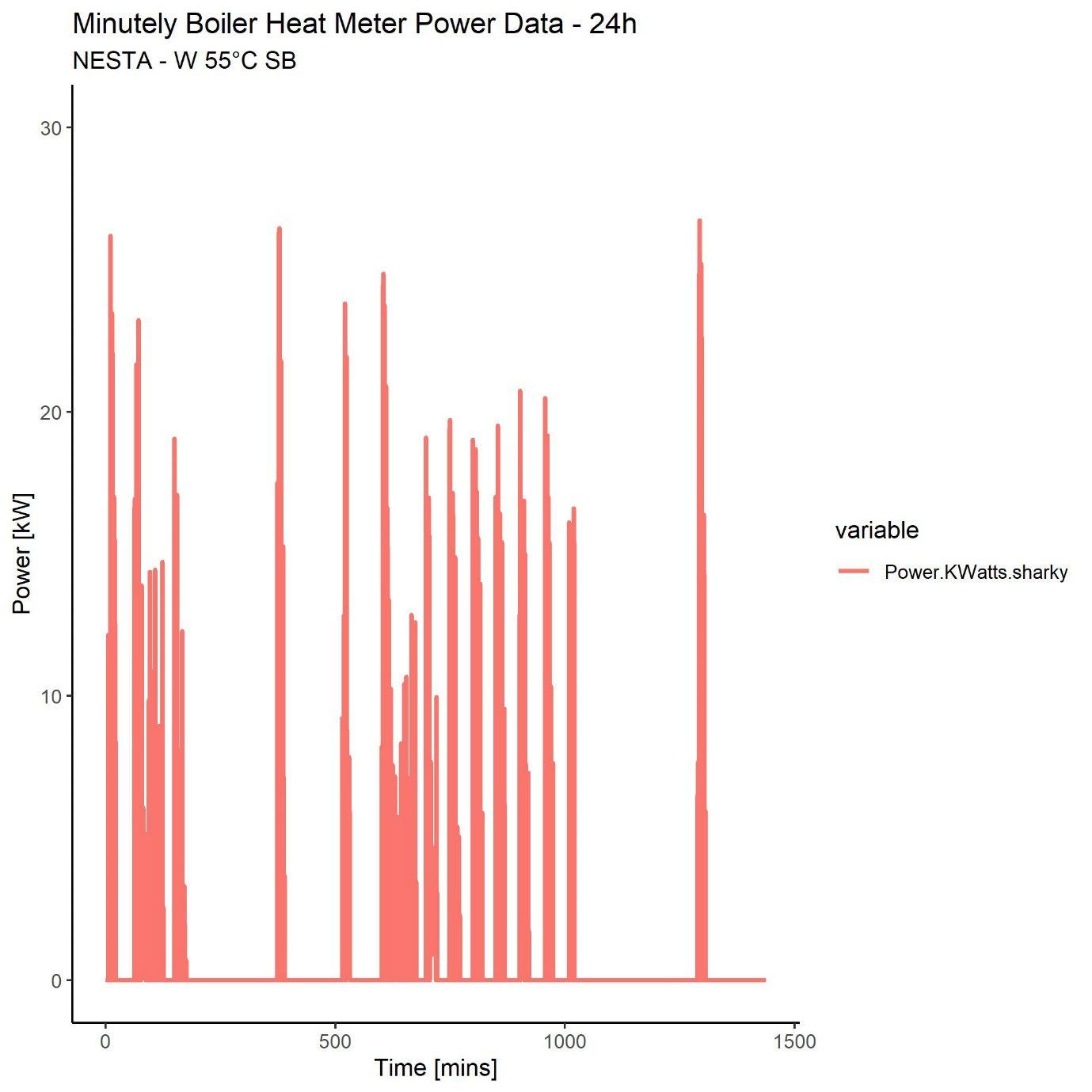
Bar chart showing minutely boiler heat meter power data over 24 hours for NESTA - W 55°C SB, with power in kW on the y-axis and time in minutes on the x-axis.
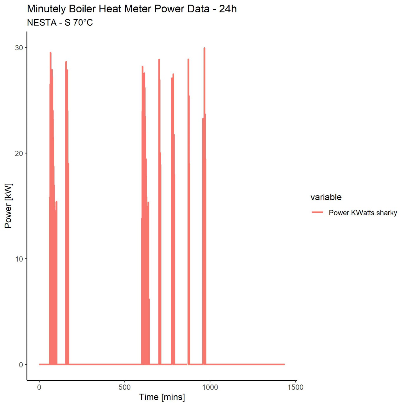
Bar chart showing minutely boiler heat meter power data over 24 hours for NESTA - S 70°C, with power in kW on the y-axis and time in minutes on the x-axis.
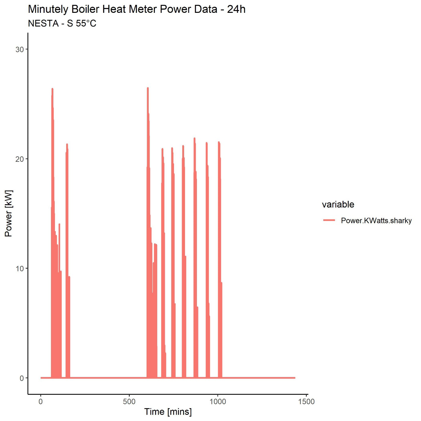
Bar chart displaying minutely boiler heat meter power data over 24 hours for NESTA - S 55°C, showing power in kW over time in minutes.
Appendix G. Internal temperature measurements
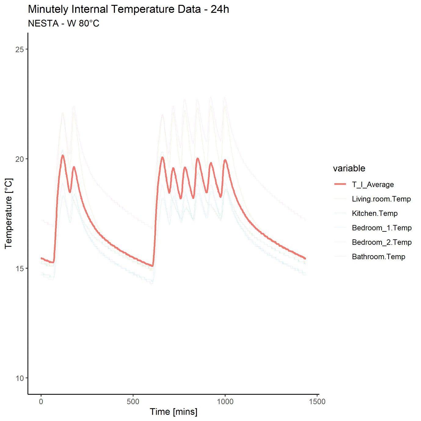
Line graph showing minutely internal temperature data over 24 hours for different rooms and an average temperature, in degrees Celsius.
Line graph showing minutely internal temperature data over 24 hours for NESTA - W 70°C, including different rooms and an average, in degrees Celsius.
Line graph showing minutely internal temperature data over 24 hours for a NESTA W 60°C system, including average and individual room temperatures.
Line graph showing minutely internal temperature data over 24 hours for a NESTA W 55°C system, including average and individual room temperatures.
Line graph showing minutely internal temperature data over 24 hours for a NESTA W 50°C system, including an average and individual room temperatures.
Line graph displaying minutely internal temperature data over 24 hours for NESTA - W 55°C SB, including average and individual room temperatures.
Line graph presenting minutely internal temperature data over 24 hours for NESTA - S 70°C, including average and individual room temperatures.
Line graph showing minutely internal temperature data for 24 hours across different rooms (living room, kitchen, bedrooms, bathroom) and the average, plotted against time in minutes.
-
A final report with confirmed uncertainties for gas consumption and boiler efficiency will follow. ↩
-
Construction details and floor plans are provided in Appendix A and Appendix B, respectively. ↩
-
Refer to Appendix C for more details of the Energy House's monitoring system. ↩
-
Gas energy consumption based on volumetric gas consumption measurement. Energy consumption (kWh) = volume (m³) * calorific value (MJ/m³) * pressure and temperature correction factor (1.02264) * 3.6 (converts Watts to kWh). Calorific values for each test period obtained from the National Grid. ↩
-
Gas meter uncertainty: ± 1.5% > 1 m³/h, ± 3% ≤ 1 m³/h. ↩
-
English housing data from Department for Levelling Up, Housing and Communities (2021) English housing survey 2020 to 2021: Headline report. London: Department for Levelling Up, Housing and Communities. Available at: gov.uk/government/statistics/english-housing-survey-2020-to-2021-headline-report ↩
-
Glew, D, Parker, J, Fletcher, M, Thomas, F, Miles-Shenton, D, Brooke-Peat, M, Johnston, D and Gorse, C (2021) Demonstration of energy efficiency potential: literature review of benefits and risks in domestic retrofit practice and modelling (BEIS Research Paper Number 2021/014). London: Department of Business Energy and Industrial Strategy. Available at: assets.publishing.service.gov.uk/government/uploads/system/uploads/attachment data/file/972027/deep-literature-review.pdf ↩
-
HTC, HLP, and AP50 are based on previous measurements taken when the fabric of the Energy House was in a similar configuration ↩
-
The SAP assumed temperate of 18 °C for the bathroom was not used as this would have resulted in the bathroom radiator being oversized and radiators in surrounding zones being undersized. ↩
-
Boiler efficiency = boiler output [kWh] / gas consumption [kWh] ↩
-
System efficiency = boiler output [kWh] / (gas consumption [kWh]+ boiler electricity consumption [kWh]) ↩
-
BEAMA - Load and Weather Compensation Test Report (2021) Available at: beama.org.uk/resourceLibrary/salford-tests-on-load-and-weather-compensation-.html ↩