Executive Summary
- Excess weight prevalence in England has increased rapidly in the last 30 years (Health Survey for England 2022). Nesta has the goal of contributing to halving the obesity prevalence in the UK by 2030 from its 2020 levels and it intends to do so by designing, testing and scaling interventions in the food environment that impact at population level.
- Obesity prevalence in the early 1990s was half that measured in 2020, so achieving Nesta's goal would be consistent with taking obesity levels back three decades.
- This study provides an estimate of the average reduction in daily calories required for the English population to lose enough weight to halve the obesity rate over the next 10 years. Future directions for this work include an assessment of the extent to which current government interventions have been able to produce a reduction consistent with the calculated target and what other food environment interventions might be considered to meet the target.
- In order to provide a population level benchmark for calorie reduction, Nesta developed a novel methodology based on the comparison of historical Body Mass Index (BMI) distributions. The methodology consists of the following steps. Firstly, the BMI distributions from 1991-92 and 2019 are equivalised using representative samples from the Health Survey of England. The equivalising exercise is to determine the average reduction in body weight that people in each BMI class (underweight, healthy weight, overweight, obese and morbidly obese) would need to experience for the BMI distribution to change its shape and location to match that of 1991-92 (when obesity prevalence was roughly half what we have today). Secondly, the reduction in daily calorie intake is calculated that each respondent of the 2019 Health Survey for England would need in order to lose enough weight to meet the target goal defined by comparing the BMI distributions in the first step. The reduction in daily calories has been calculated using the model developed by Hall et al. (2011), which is considered the gold standard in the field and it was also the basis of the Department for Health and Social Care's Calorie Model (Department of Health and Social Care 2018).
- The reduction in calories required for individuals with excess weight (BMI higher than 25 kg/m2) in England is around 8.5% of current intake for both females (190 kcal/day) and for males (241 kcal/day). When results are broken down by BMI group within the excess weight group, there is variation in the calorie reduction required. The required reduction is larger for higher BMIs with figures for overweight males being at 6.9% (187 kcal/day), obese males at 10.3% (307 kcal/day) and morbidly obese males at 14.8% (531 kcal/day). For females, the figure for overweight categories is a 6.5% reduction (136 kcal/day), for obese ones is 9.6% (222 kcal/day) and for morbidly obese groups is 13.7% (395 kcal/day). Under the assumption of no change in daily intake for underweight and healthy weight BMI groups, at population level and across all BMI groups these figures translate to an average of 165 kcal/day for males and 115 kcal/day for females.
- The reduction in calories are calculated within a timeframe of three years and for groups of individuals in separate BMI categories and for the group of people with excess weight as a whole (overweight, obese and morbidly obese). Population level figures are also provided under the assumption that BMI groups in the underweight and healthy weight categories do not change calorie intake.
- The benefits of halving obesity to the economy are large. A recent study calculated that the annual cost of adult obesity to UK society is around £54bn (Frontier Economics 2022). Based on this figure, halving obesity prevalence would save around 300,000 Quality Adjusted Life Years every year (one QALY is one year of life in perfect health). Using the government's estimate of the monetary value of a single QALY (£70,000) these QALY savings are equivalent to a monetary value of around £20 billion. The cost savings to the NHS are calculated to be around £3.25 billion.
- Whilst acknowledging the difficulty of synthesising complex biological processes in tractable equations and of collecting anthropometric measurements at large scale, this study uses gold standard methods and the most up to date and comprehensive dataset for England to produce a robust figure for calorie reduction at population level, and across BMI groups.
Background
Excess weight prevalence in England has increased rapidly in the last 30 years (Health Survey for England 2022). In 2007 the UK Government's Foresight Programme commissioned a report which included projections of prevalence of obesity for the subsequent 40 years. The modelling was conducted with data from the 1990s and early 2000s and it predicted large and sustained increases in excess weight prevalence (McPherson, Marsh, and Brown 2007). However, more recent studies suggest that the rapid rises in excess weight prevalence may be slowing but prevalence of very high BMI (above 35 kg/m2) is set to continue increasing (Abarca-Gómez et al. 2017; Cobiac and Scarborough 2021). The most recent review conducted for England shows that the proportion of the population that is overweight or obese will likely remain stable in the next 10 years (Cobiac and Scarborough 2021). Regardless, the evidence shows that the majority of the English population is predicted to continue living with excess weight in the next 10 years.
While the projections from these models provide useful background, they only extrapolate from current macro trends in excess weight prevalence. They make no reference to population level calorie intake or social/educational factors that directly and indirectly influence people's health behaviours, driving differences between subgroups' BMI distribution trajectories. Therefore, the findings from these projections are less useful as analytical tools to determine how changes in diets may impact upon obesity prevalence. More generally, an understanding of the connection between dietary behaviours and excess weight prevalence will help Nesta prioritise between different food environment interventions and will provide a guide of the overall scale of intervention needed to meet the A Healthy Life mission's goal. To link excess weight prevalence to diets we make use of formulas developed within weight loss analysis which provide a way of linking current BMI estimates with daily calorie intake (Hall et al. 2011).
Research Question
Nesta has the goal of achieving a 50% reduction in obesity prevalence by 2030 compared to 2020 levels. This is an ambitious goal and it has the aim of focussing and galvanising Nesta's work programme. The goal of halving obesity prevalence is consistent with bringing obesity levels back to those measured in 1991/92 in England. The timeline of Nesta's strategy is between 2020 and 2030; the Health Survey for England (HSE) was discontinued in 2020 due to the COVID pandemic, so the wave of 2019 is considered instead. It is clear that according to current trends halving the prevalence of obesity by 2030 will not happen without effective and population-wide interventions.
The aim of this work is to investigate the scale of intervention required in terms of reduction in daily calorie intake by addressing the questions: How many fewer calories would people living with excess weight need to eat on average to ensure halving obesity prevalence in England?
Definitions
To begin understanding the scale of the challenge it is useful to consider how the obesity epidemic has come about in the first instance. There is substantial evidence that current levels of excess weight prevalence have come about via small daily discrepancies in energy intake and expenditure which have resulted in gradual energy accumulation and weight gain, with reductions in physical activity levels being a secondary factor (Hill, Peters, and Wyatt 2009, Scarborough et al. 2011).
According to Hill, Peters, and Wyatt (2009) “the term energy gap was created to estimate the degree of change in the energy balance point (the absolute energy intake and expenditure at which balance is reached [i.e. body weight becomes stable]) required for success in body weight goals” (p. 2). It should be noted that there is not a full consensus on the exact definition of energy gaps and the ways in which they can be measured (for a review see Schutz et al. (2014) and Millward (2013)). Nevertheless, following the framework laid out by Hill, Peters, and Wyatt (2009) this study provides a methodology and estimates the energy maintenance gap for England that would bring about a reduction of obesity levels by 50% compared to 2019.
The energy maintenance gap provides an estimate of how much energy requirements change with weight loss, which in turn, provides an estimate of how much energy balance must be changed for a person to attain and maintain a new, lower body weight. It can be achieved through increased physical activity, reduced calorie intake or a combination of both: the focus of this study is reduction of calorie intake so changes in physical activity levels are not considered. The energy gap for weight loss maintenance can be calculated using a regression model linking energy requirements with body weight. Using such regression equations, it has been pointed out that the energy gap required to go from a very obese state to a non-obese state is large because the decrease in intake needs to be large enough to offset the large amount of energy that is accumulated in people's bodies in the form of fat from decades of slow weight gain (Hill, Peters, and Wyatt 2009). Moreover, there is a time component to weight loss, as when intake is reduced it takes months or years for a new stable state to be achieved and the progress of weight loss slows with time.
Methods
The chosen approach requires first to calculate body weight targets by comparing the changes in average body weight in the English population between 1991-92 and 2019. These body weight targets are computed to use for calculating the energy maintenance gap which is the amount of permanent daily reduction in calories that is needed for an individual to reach a given target body weight. The energy maintenance gap is computed using the formulas developed by Hall et al. (2011).
Calculating Body Weight Targets
The reference years of 1991-92 have been chosen because in the early 1990s the obesity prevalence in England was half that of 2019. This choice is consistent with Nesta's strategic goal of halving obesity prevalence by 2030.
Body weight targets are calculated by first equating the BMI curves of 1991-92 and 2019 according to relevant percentiles (those defining the BMI categories of underweight, healthy weight, overweight, obese and morbidly obese) and then calculating the average body weight in the same percentile ranks of the distribution.
To equate the distributions, starting from the BMI distribution of 2019 the share of individuals that belong to each BMI category is calculated and these shares are used to define new 'equated' BMI thresholds for the 1991-92 distribution. For example, 3.34% of individuals from the 2019 sample have BMI higher than 40 (they are morbidly obese); in 1991-92 the BMI cut off that characterises the 3.34% of the population with the highest BMI is 35.2. Hence, the 1991-92 'equated' obesity BMI cut off is 35.2 (rather than 40).
Target body weights are defined as a percentage reduction of current weight. For example, after having equated the two BMI distributions it is found that on average body weight of obese women was 11.7% lower in 1991-92 compared to 2019; therefore, the target weight of all obese women in 2019 is set to be 11.7% lower than their current weight.
Calculating the Energy Maintenance Gap
The energy maintenance gap is calculated using the model developed by Hall et al. (2011) and operationalised by researchers at the National Institute of Public Health of Mexico in the open source R package bw. The model by Hall is considered the gold standard for modelling individual changes in body weight as a result of modification in calorie intake. It is a dynamic mathematical model of body weight change that simulates how diet changes affect body glycogen and body fluids (published as supplemental material to Hall et al. 2011). The formulas underpinning this model were also the basis of the Department for Health and Social Care's Calorie Model (Department of Health and Social Care 2018) and are used internationally by public sector organisations (such the United States Department of Agriculture (Lin et al. 2011)), academia (e.g. Choi, Seligman, and Basu 2017; Long et al. 2015) and the consultancy sector (Dobbs et al. 2014). Baseline values of total energy expenditure of all sample respondents is calculated from body weight, height, sex and age data as a proxy for intake using Mifflin et al. (1990) formulas (see equation 1).
The equations outlined by Hall et al. (2011) are used to simulate alternative distributions for body weight and BMI based on the composition of the 2019 HSE sample and compute the calorie intake that is consistent with the body weight distribution. The difference in calorie intakes by BMI groups between the actual and simulated 2019 distributions provides the estimate for the energy maintenance gap.
The timeline for weight loss is 3 years. This decision is supported by Hall et al. (2011) who find that 95% of the total weight change from a one-off permanent reduction in calorie intake happens within 3 years (page 9).
Validation Steps
Validation checks are run to consider to what extent the methods used achieve the eventual goal of shifting the BMI distribution of 2019 to halve obesity prevalence. To do this we compare graphically the simulated 2019 distribution and the 1991-92 distribution which the simulation is set out to replicate and we report the distribution of BMI categories calculated from actual and simulated 2019 data.
Data
The Health Survey for England (HSE) is an annual cross-sectional survey of a nationally representative random general population sample in England (Health Survey for England 2022). The survey monitors the trends in the nation's health and care. It started in 1991 and has been carried out annually since then. The HSE includes adults aged 16 and over (since 1995 it has also included children aged 2-15). Each year the HSE includes a set of core questions on general health, psycho-social indicators, demographic and socio-economic indicators, and measurements of height and weight. Measurements of height and weight are collected as part of the main interviewer visit.
In this analysis two HSE waves are selected: 1991-92 and 2019 (the HSE was discontinued in 2020 for a year due to the COVID pandemic). While the first data collection happened in 1991, the first published wave is for 1991 and 1992 combined. Survey weights are not available for 1991-92 and the documentation states that at this time they are not needed as the sample is representative of the underlying population. Survey weights for the 2019 wave are provided and used throughout the analysis. The weights take account of selection and non-response.
Table 1 contains the list of variables that have been used in the analysis.
The variables are selected to ensure comparability across survey waves and validity of measurement. Only weights and heights that are validated by the interviewer are used, with the exception of body weights that are higher than 130 kg which are reported as estimated weights in the HSE. There is a discrepancy in the way in which age is reported across the two waves: in 1991-92 age at last birthday is reported, but this has been removed from the available 2019 wave and replaced by a grouped variable. For 2019, the mid-point of the 5-year age groups is taken as the estimated age for each respondent.
Table 2 contains summary statistics for the variables included in the analysis. Figures for BMI class prevalence are reported with and without age standardisation. There has been an increase in the prevalence of excess weight between 1991-92 and 2019 which is only partially explained by population ageing. For example, the prevalence in obesity increased from 13.5% in 1991-92 to 24.7% in 2019, and only 0.9% of this increase is explained by an overall ageing of the population. In other words, if the age distribution had remained the same as 1991-92 the prevalence of obesity in 2019 would be 23.8%.
Table 1 - Variables List
| Variable |
HSE name |
Description |
HSE name |
Description |
| Sex |
sex |
Respondent's sex at birth |
Sex |
Respondent's sex at birth |
| Age |
age |
Age at last birthday |
Age35g |
Age, 3 year bands for 0-15, 5 year bands 16+ |
| Weight |
wtvalid |
Valid weight (kg) including estimated > 130 kg |
WtVal |
Valid weight (kg) including estimated > 130 kg |
| Height |
htvalid |
Valid height |
HtVal |
Valid height |
| BMI |
bmivalid |
|
BMIVal |
|
| Survey weight |
|
|
wt_int |
Weight for analysis of core interview sample |
Table 2 - Summary Statistics
|
HSE 1991-92 |
HSE 2019 |
|
Mean/Proportion |
Standard Deviation |
| % Female |
52.4% |
|
| Age |
45.0 |
18.0 |
| Weight |
71.9 |
14.8 |
| Height |
167.6 |
9.7 |
| BMI |
25.6 |
4.6 |
| BMI Class |
|
|
| % Underweight |
2.1% |
|
| % Normal |
48.7% |
|
| % Overweight |
35.0% |
|
| % Obese |
13.5% |
|
| % Morbidly Obese |
0.7% |
|
| Total (weighted) |
6544 |
|
Notes: Health Survey for England waves 1991-92 and 2019. Author's calculations. All figures for 2019 have been calculated using survey weights (wt_int). Survey weights are not available for 1991-92.
Results
In the first section estimates of body weight targets based on a comparison of the BMI distributions of 1991-92 and 2019 are reported. The choice of survey waves is based on the modelling approach of shifting the BMI curve of 2019 to the shape and location of that in 1991-92, when obesity prevalence was half that observed in 2020. In the following section estimates for the the energy maintenance gap for the obese population for England are reported. The energy maintenance gap is the amount of permanent daily reduction in calories that is needed for an individual to reach a given target body weight.
Body Weight Targets
The starting points are the BMI distributions for 1991-92 and 2019, for males and females separately. Males and females are considered separately because the analytical formula for total energy expenditure are different depending on sex.
Figures 1 and 2 report the BMI distributions for males and females separately in 1991-92 and 2019.
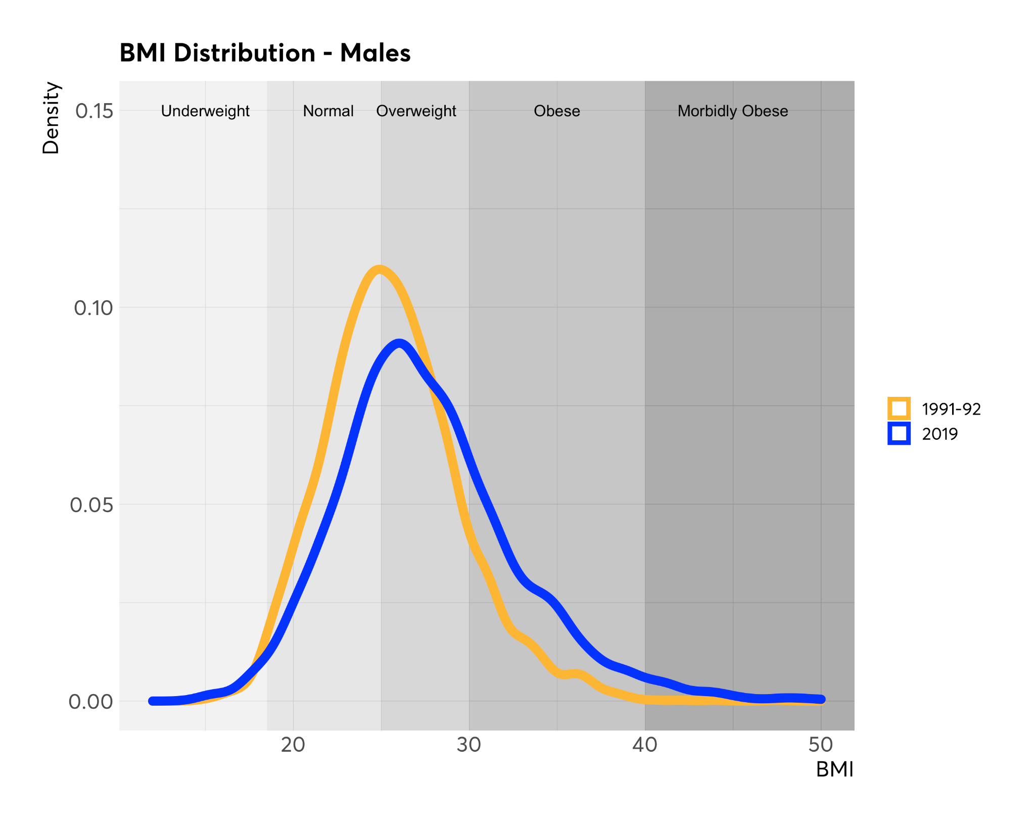
Figure 1 - BMI distribution by survey year for males
Notes: Distribution of BMI for males from Health Survey for England waves 1991 and 2019. Author's calculations. All figures for 2019 have been calculated using survey weights (wt_int).
Survey weights are not available for 1991.
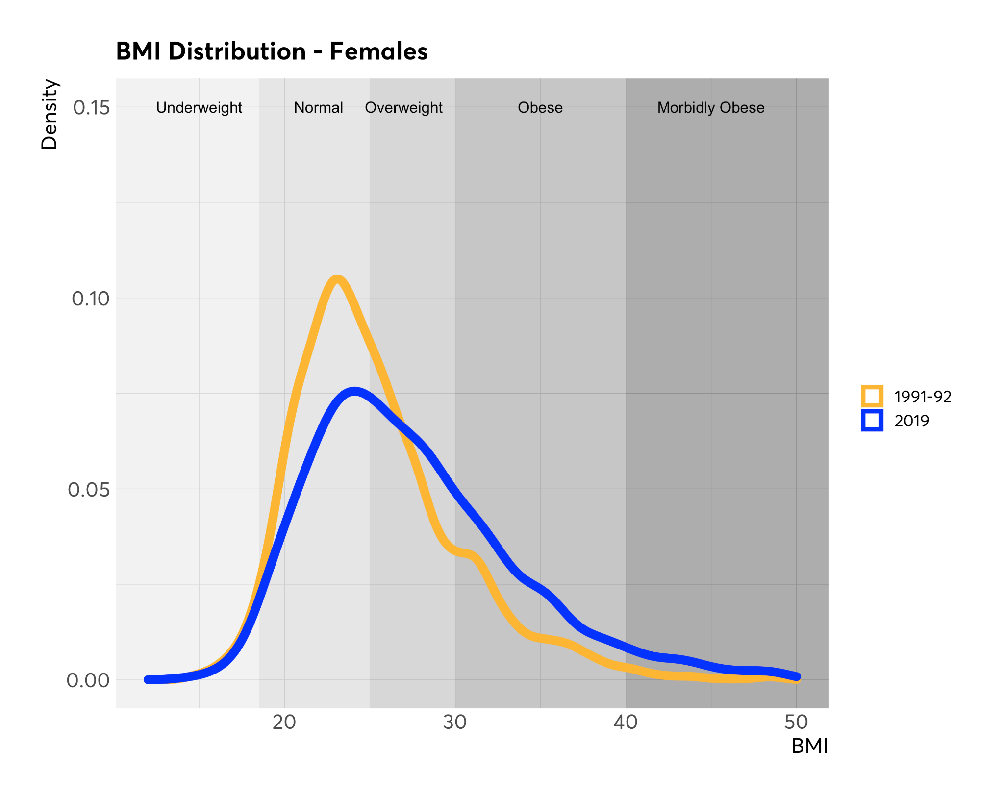
Figure 2 - BMI distribution by survey year for females
Notes: Distribution of BMI for females from Health Survey for England waves 1991 and 2019. Author's calculations. All figures for 2019 have been calculated using survey weights (wt_int). Survey weights are not available for 1991.
The inspiration behind the methodology comes from the practice of equipercentile equating which is commonly applied in the context of educational assessment (Livingston 2014). The idea is to find the values of the BMI distribution in 1991-92 which have the same percentile rank as the BMI values used as cut offs for defining excess weight in the 2019 distribution.
Table 3 - Equated BMI Cut-Off
| BMI class |
2019 cut-off |
1991-92 cut-off |
| Underweight |
<18.5 |
<18.4 |
| Normal |
18.5 - 24.9 |
18.4 - 23.5 |
| Overweight |
25 - 29.9 |
23.6 - 27.4 |
| Obese |
30 - 39.9 |
27.5 - 35.2 |
| Morbidly obese |
>= 40 |
>= 35.3 |
Notes: Health Survey for England waves 1991-92 and 2019. Author's calculations. All figures for 2019 have been calculated using survey weights (wt_int). Survey weights are not available for 1991-92.
Population target body weight are determined as the percentage difference in mean body weight for each BMI rank among the excess weight groups and sex (Table 6). This is defined in terms of the percentage weight reduction needed to align the average population body weight of 2019 to that of 1991-92 as calculated from equating the BMI curves for the two survey years.
Table 4 - Body Weight by Excess Weight BMI Group
| | 1991-92 | 2019 | Difference |
|:-------------------------------------|:----------|:----------|:----------|:----------|:----------|:----------|:----------|:----------|:----------|
| | Median | Mean | St. Dev. | Median | Mean | St. Dev. | Mean | % Median | % |
| BMI cumulative rank [35.8% - 72.0%) - 2019 Overweight category | | | | | | | | | |
| Females | 65.0 | 65.5 | 6.1 | 71.0 | 70.8 | 7.0 | 5.3 | 8.1% | 6.0 | 9.2% |
| Males | 77.0 | 77.5 | 7.2 | 84.0 | 84.3 | 8.4 | 5.3 | 8.7% | 7.0 | 9.1% |
| BMI cumulative rank [72.0% - 96.7%) - 2019 Obese category | | | | | | | | | |
| Females | 78.0 | 77.8 | 8.4 | 86.0 | 86.8 | 9.9 | 9.0 | 11.7% | 8.0 | 10.3% |
| Males | 90.0 | 90.6 | 9.4 | 102.0 | 102.4 | 11.8 | 11.8 | 13.0% | 12.0 | 13.3% |
| BMI cumulative rank [96.7% - 100%] - 2019 Morbidly Obese category | | | | | | | | | |
| Females | 98.0 | 101.4 | 17.6 | 115.0 | 118.0 | 16.0 | 16.6 | 16.4% | 17.0 | 17.3% |
| Males | 114.0 | 115.1 | 14.8 | 136.0 | 136.2 | 18.2 | 21.1 | 18.4% | 22.0 | 19.3% |
Notes: Health Survey for England waves 1991-92 and 2019. Author's calculations. All figures for 2019 have been calculated using survey weights (wt_int). Survey weights are not available for 1991-92. Mean refers to arithmetic mean.
It should be noted that this is not a longitudinal analysis therefore the weight of individuals is not tracked over time and there are individuals in each category in 2019 that were not alive in 1991-92. The assumption behind the inference is therefore the one of extrapolating between groups that have the same rank position on the BMI distribution.
Energy Maintenance Gap
The baseline calorie intake is calculated for each survey respondent by first working out their Resting Metabolic Rate (RMR). To calculate RMR the formula proposed by Mifflin et al. (1990) is used. To derive the Total Energy Intake (TEE) (which is assumed to be equal to Total Energy Expenditure (TEE) at baseline) a physical activity factor of 1.6 is used, which describes a moderately light level of physical activity and it is consistent with the value used for calculating the Dietary Reference Values for Energy in the UK (Scientific Advisory Committee on Nutrition 2012). The formulas are a function of body weight (W), height (H) and age (A) and are defined for males (TEEM) and females (TEEF) separately as
TEEF = 1.6 · (10· W + 6.25 · Η − 5 · A - 161)
ТЕЕM = 1.6 · (10 · W + 6.25 · H − 5 · A + 5)
(1)
The distribution of intake in 1991-92 and 2019 for males and females across the whole population is reported in Figure 3. By shifting the BMI distribution from 2019 to 1991-92 levels the intake distribution would also shift to levels of 1991-92 as it is a function of body weight and height. The minimum and maximum observed body weights for females are 34.1 kg and 182.0 kg which correspond to implied intakes of 1360 kcal/day and 3950 kcal/day respectively. For males, the minimum observed body weight is 37 kg which corresponds to an implied intake of 1844 kcal/day and the maximum observed weight is 182.4 kg which corresponds to a 4534 kcal/day implied intake.
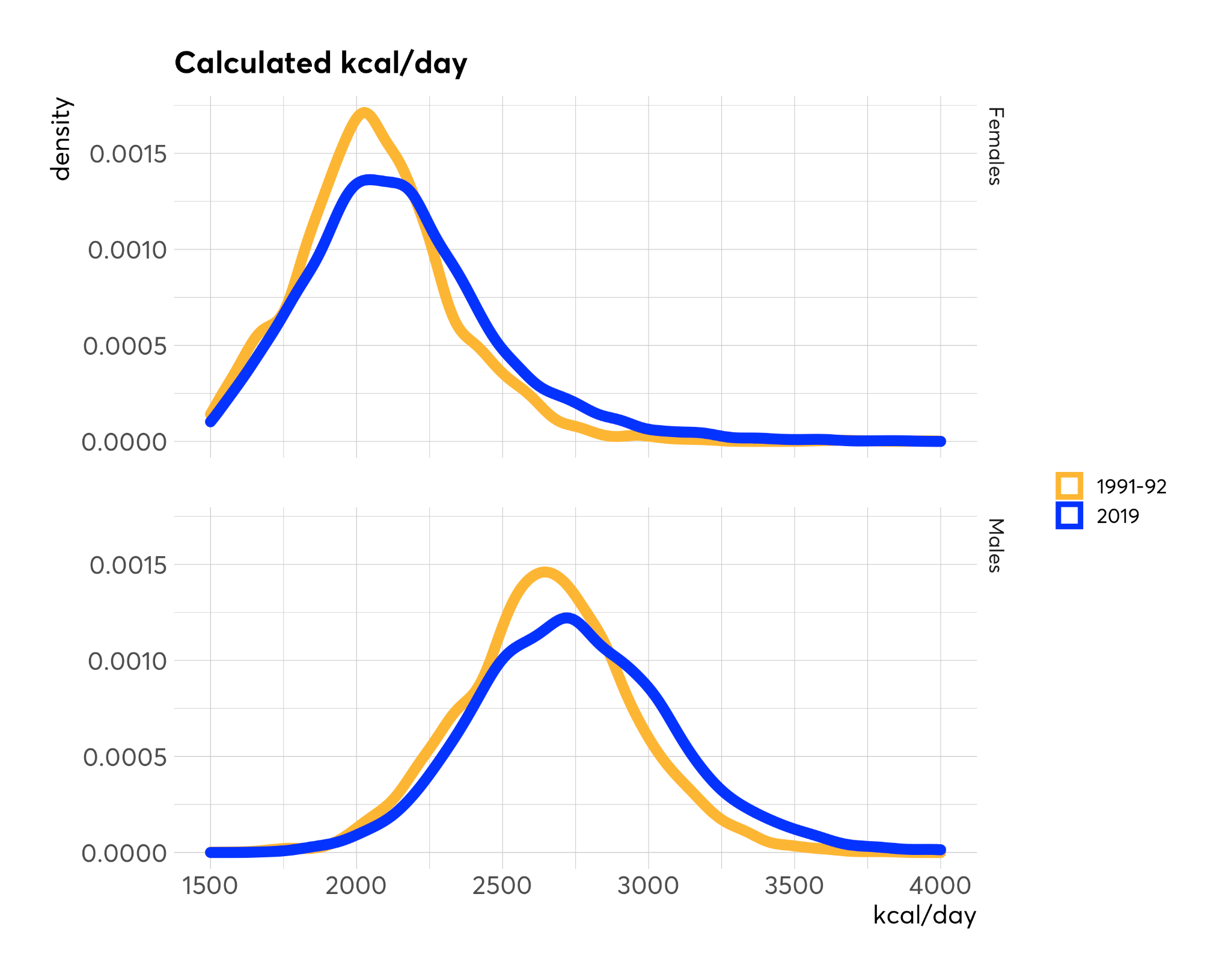
Figure 3 - Calculated intake distribution for females (above) and males (below) by survey year
Notes: Health Survey for England waves 1991 and 2019. Author's calculations. All figures for 2019 have been calculated using survey weights (wt_int). Survey weights are not available for 1991.
Secondly the model developed by Hall et al. (2011) is applied to calculate the change in intake as a percentage of current intake required to meet the body weight goals previously defined. The model is applied to every sample respondent. We defer to Hall et al. (2011) for full details of the model.
The Maintenance Energy Gap is defined as the difference between the baseline intake and that resulting from the calorie reduction necessary to lose and maintain the new current lower body weight.
Figure 4 displays the shift in the intake distribution resulting from the reduction in intake by sex and BMI group and Table 5 contains high level summary with full details of summary statistics in Table 6. The population level figure is calculated under the assumption of no change in intake for the underweight and healthy weight groups. At population level, the Maintenance Energy Gap is estimated to be 115 kcal/day for females and 165 kcal/day for males (5.4% and 6.0% of current intake respectively). Due to the skew in the distribution of the intake difference, the population level figures should not be interpreted as the value required for any actual individual. However, they are an important and useful benchmark for any calorie reduction intervention because calorie intake and calorie purchased can much more easily be monitored at population level via for example retailer and manufacturer data or barcode scanner data (Dubois, Griffith, and O'Connell 2022).
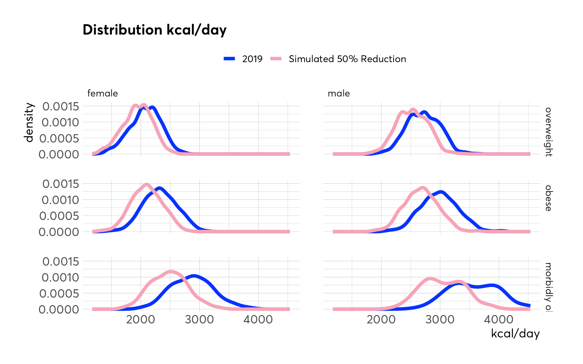
Figure 4 - Daily Intake Distribution for Females (left) and Males (right) - Current and under the 50% Obesity Reduction Scenario
Notes: Health Survey for England wave 2019. Author's calculations. All figures for 2019 have been calculated using survey weights (wt_int).
The figures are larger for excess weight groups, standing at 190 kcal/day for females and 241 kcal/day for males (both 8.5% of current intake). Within the excess weight groups, the figures are larger for larger BMIs: for obese females, the Maintenance Energy Gap is 222 kcal/day which is a 9.6% reduction compared to the intake calculated from the 2019 distribution. For obese males the relevant figure is 307 kcal/day which is a 10.3% reduction compared to the intake in the 2019 HSE sample. For overweight groups, the figures are 6.5% for females and 6.9% for males and for morbidly obese are over 13%.
Table 5 - High Level Summary of Energy Maintenance Gap by Sex and BMI Group
| BMI group |
Females |
Males |
|
kcal/day |
% reduction |
| Overweight |
136 kcal/day |
-6.5% |
| Obese |
222 kcal/day |
-9.6% |
| Morbidly Obese |
395 kcal/day |
-13.7% |
| Excess Weight |
190 kcal/day |
8.5% |
| Population* |
115 kcal/day |
-5.4% |
Notes: * The population level figure is calculated under the assumption of no change in intake for the underweight and healthy weight groups. This figure is reported as a useful benchmark for monitoring calorie reduction progress, as figures for calorie consumed or purchased are more easily available at whole population level and figures for subgroups cannot be estimated accurately.
Figure 5 shows the distribution of percentage differences. These are the estimated values of percentage reduction in intake required among individuals to meet the target weight reduction defined in Table 6. Most respondents within the same BMI group have similar calorie reduction values. The interquartile ranges for females are 0.4%, 0.5% and 0.7% for overweight, obese and morbidly obese groups respectively. For males, the relevant values are 0.2%, 0.3% and 0.5%. These values tell us the percentage point difference in the calorie reduction for the middle 50% of the sample. For example, for obese females, the middle 50% of the sample have all calorie reduction values between -9.3% and -9.8% which correspond to a reduction of -237 kcal/day and -207 kcal/day.
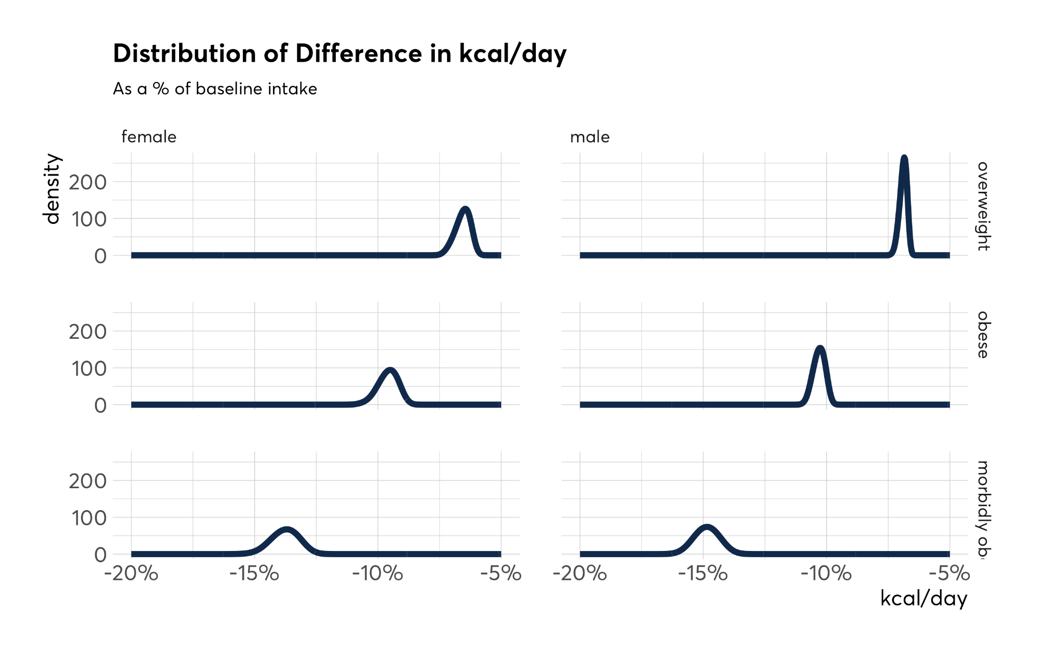
Figure 5 - Distribution of Percentage Reduction in Daily Intake for Females (left) and Males (right) under Scenario of 50% Obesity Reduction
Notes: Health Survey for England wave 2019. Author's calculations. All figures for 2019 have been calculated using survey weights (wt_int).
Table 6 - Projected Required Mean Daily Intake for Excess Weight Groups
|
Before |
After |
Difference |
95% CI |
% Difference |
| Overweight |
|
|
|
|
|
| Males |
2711 |
2525 |
-187 |
(-188, -185) |
-6.9% |
| Females |
2079 |
1943 |
-136 |
(-137, -135) |
-6.5% |
| Obese |
|
|
|
|
|
| Males |
2987 |
2679 |
-307 |
(-309, -305) |
-10.3% |
| Females |
2325 |
2103 |
-222 |
(-224, -221) |
-9.6% |
| Morbidly Obese |
|
|
|
|
|
| Males |
3575 |
3044 |
-531 |
(-548, -514) |
-14.8% |
| Females |
2876 |
2481 |
-395 |
(-403, -388) |
-13.7% |
| All Excess weight Groups |
|
|
|
|
|
| Males |
2839 |
2598 |
-190 |
(-245, -238) |
-8.5% |
| Females |
2239 |
2598 |
-241 |
(-194, -187) |
-8.5% |
| Population |
|
|
|
|
|
| Males |
2753 |
2588 |
-165 |
(-179, -159) |
-6.0% |
| Females |
2129 |
2014 |
-115 |
(-119,-111) |
-5.4% |
Notes: Health Survey for England wave 2019. Author's calculations. All figures for 2019 have been calculated using survey weights (wt_int). Mean is arithmetic mean.
Validation
A first validation check involves the comparison between the BMI distribution from the 1991 HSE and that simulated in this study (Figure 6). Given that the exercise was intended to replicate a shift in the BMI distribution, the chart provides a visual check of the extent to which the shift has been achieved. The plot shows indeed a high degree of congruence.
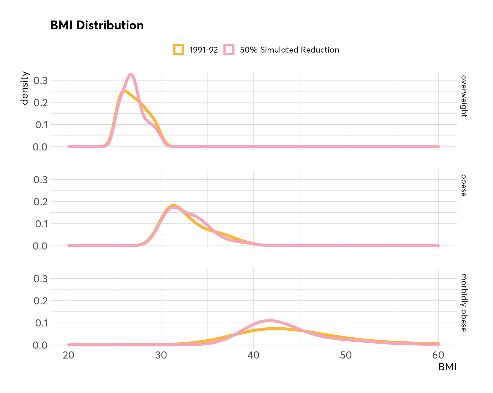
Figure 6: Comparison of BMI Distributions for the 1991 HSE sample and the simulated 2019
Notes: Health Survey for England waves 1991 and 2019. Author's calculations. All figures for 2019 have been calculated using survey weights (wt_int). Survey weights are not available for 1991.
The excess weight prevalence resulting from the exercise of simulating a BMI shift is displayed in Figure 7. To produce this figure, the assumption that there is no difference in intake of populations with normal and underweight BMI categories is made, while all other categories reduce intake to the level of the energy maintenance gap estimated in this study. The obesity rate drops from 24.7% to 11.4%. The target of halving obesity by 50% is overshot slightly: a possible explanation is the use of a unique percentage reduction for the whole population. Due to the skew of the body weight distribution it is likely that the calculated average change in body weight is overestimated. The percentage of population that are in the overweight category reduces from 36.2% to 34.1%, while there is a large decrease in the share of morbidly obese from 3.3% to 0.6%. The share of the population with normal weight increases significantly from 33.9% to 52.1%, while the share of underweight remains unchanged.
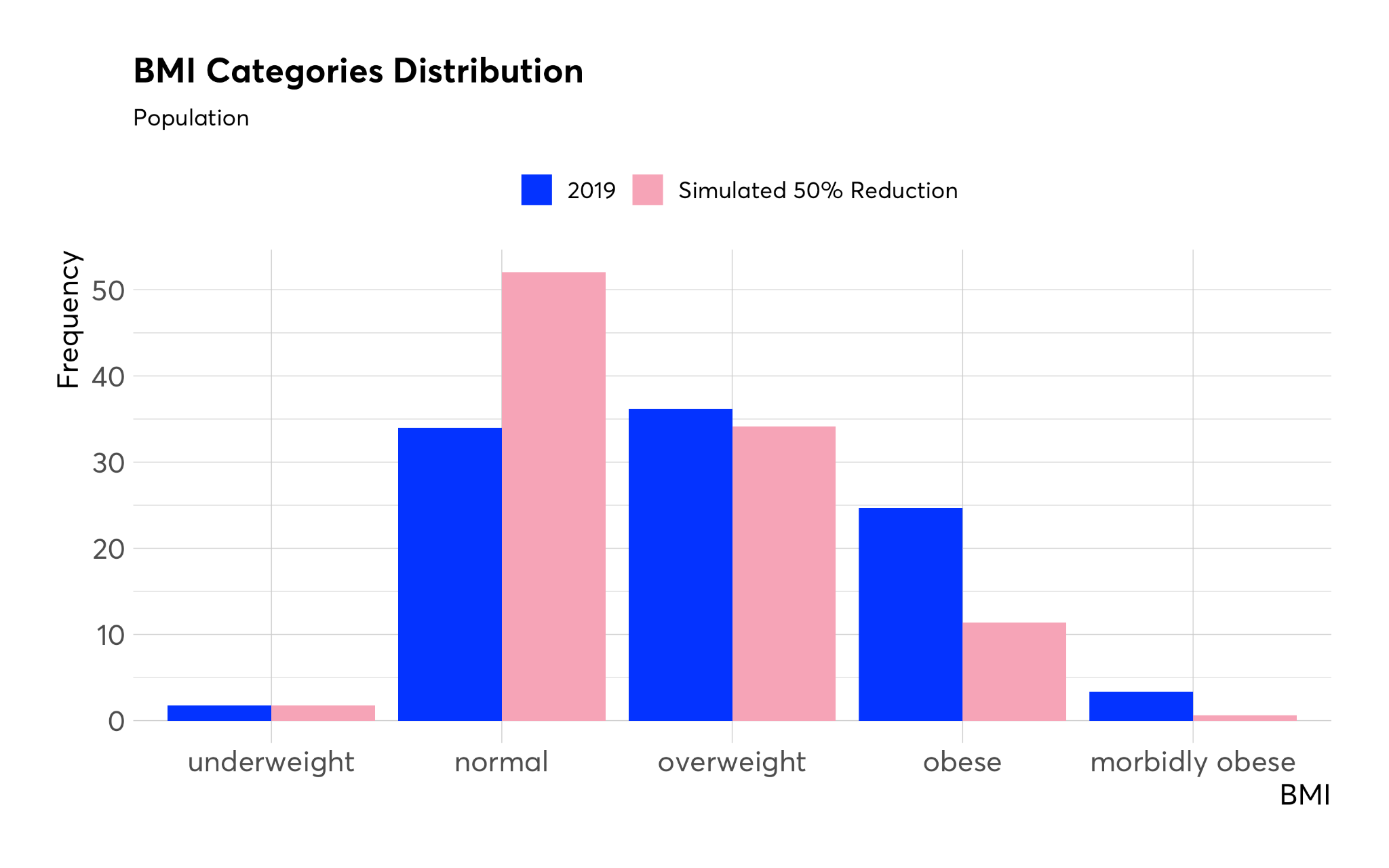
Figure 7 - Comparison of BMI Categories Distribution
Notes: Health Survey for England wave 2019. Author's calculations. All figures for 2019 have been calculated using survey weights (wt_int).
Limitations
In this study we have simulated the change in daily calories intake needed for the English population BMI distribution to change position and shape to resemble that of 1991-92. The overall aim of the study is to provide context for Nesta's goals, however it is also a methodological contribution for anyone wishing to calculate energy gaps for a specific population or subgroup. Nevertheless, there are a series of limitations stemming from the methods and the data used.
The methodology in this study relies on equating the 1991-92 and 2019 BMI distributions. This procedure assumes that the composition of the populations remains relatively stable with respect to factors that are closely associated with BMI, which may not be true. For example, it has been observed that in western countries BMI increases with age, therefore a significant increase in age in 2019 compared with 1991-92 would increase BMI even in the presence of stable BMI distributions within age groups and lead to overestimating the degree of weight change needed for equating the distributions. The relationship between BMI and age is such that the estimated calorie changes are likely to be an overestimate because the population of 2019 is on average older and heavier than that of 1991-92 and part of the higher weight is explained by older age rather than weight differences between people of the same age groups. Further development of this work may include age-standardised estimates of the calorie reduction benchmark. Another factor potentially affecting the comparability between 1991-92 and 2019 is the change in the ethnic makeup of the English population which has seen the share of white British population reduce (Office for National Statistics 2022). The relationship between ethnicity and BMI is complex and further developments of this work may investigate the implications of setting calorie reduction targets for a population with evolving ethnic composition.
The model for calculating the Maintenance Energy Gap used in this exercise was developed to be used in clinical settings and for monitoring weight loss interventions on an individual basis. Therefore it does not take into account population level dynamics and it makes the implicit assumption that a population is the sum of its individuals which does not hold in reality, given the fluidity in the population make up. For example, due to the observed relationship between BMI and age explained earlier, a longitudinal study of adults will inevitably show weight gain even in cases where a population as a whole might be weight stable (or even decreasing in weight). This is typically the result of lean young people entering the adult population at the same time as heavier older people leave the population when they die (Hall et al. 2011). Moreover, there is the assumption that individuals are on a stable weight trajectory at baseline; this is unlikely to have held until now given the increase in obesity prevalence.
In addition, energy requirements cannot be measured with a precision better than 5% because the equations formulated do not fully take into account the inter-individual variability that is observed in Doubly Labelled Water data (Schoeller and Fjeld 1991). Even small initial uncertainties can lead to large expected long-term inter-individual variability of weight change (Hall et al. 2011; Schoeller and Fjeld 1991). The model also makes the assumption of a constant level of physical activity across the whole population, while in reality studies have shown that BMI and physical activity are inversely associated (Bradbury et al. 2017).
An additional and significant limitation is the analytical choice of using one single (proportional) weight target for the whole obese sample. The two main issues with this choice are that the target is not necessarily representative of the whole group and due to the skew of the body weight distribution the proportional target reduction is likely biassed upwards (compared to the alternative scenario of setting individual weight loss targets). As a result, the distribution of BMI categories overshoots the initial target of halving the obesity rate. Further development may consider more fine grained subgroups of the obese population for defining body weight targets.
The data used are samples from the Health Survey for England from survey years 1991-92 and 2019. Although this is the best data source available for measures such as body weight and height, its representativeness with respect to anthropometric measurements has not been fully assessed. In other words, while it is possible to assess that the HSE sample is representative of the English population with respect to e.g. age and gender because the population distribution for these variables is known, a population distribution for BMI is not available and therefore it is necessary to make the assumption that the representativeness with respect to other characteristics would carry forward to weight and height. There have been some suggestions that because height and weight measurements are collected during an interviewer visit which respondents need to agree to, respondents who are older and in poorer health are less likely to consent to their measurements being taken and might be underrepresented in the HSE sample (Amies-Cull et al. 2022). Because of the positive relationship between age and BMI this would result in BMI estimates from the HSE sample being biassed downwards and the bias is likely to be larger for more recent waves due to an ageing population.
This report has focussed on population level estimates. It is attractive to consider a single population figure as a target for calorie reduction when devising policies and interventions. However, it should be noted that using a single population figure without understanding implications for subgroups masks potentially large distributional effects. For example, living in an area of high deprivation and ethnicity are two factors that strongly interact with obesity and that are likely to be important when considering distributional effects (Gatineau and Mathrani 2011; Health Survey for England 2022).
When considering different ethnic groups, it is known that BMI cut-offs for equivalent BMI-RR disease outcome relationships for non-white subgroups are lower (Caleyachetty et al. 2021). Therefore a single population benchmark which is based on BMI cut offs that are defined for the white population would not represent the accurate situation of minority groups.
Given the known relationship between living in a deprived area and obesity prevalence, people at the top end of the BMI scale are more likely to be from more deprived communities. Therefore, calorie reductions around the population level benchmark figure would be insufficient for halving obesity prevalence in communities with high baseline excess weight prevalence. Nevertheless, health gains from losing weight are higher for larger levels of starting BMI as shown by the non-linear relationship of BMI and Risk Ratios (RR) for non communicable diseases (Dudina et al. 2011). Therefore, a single population level benchmark figure would result in people with larger BMIs losing higher amounts of body weights than people at the lower end of the BMI scale and also experiencing a larger overall improvement in health profiles which is a reduction in health inequalities.
Discussion and Conclusions
The analysis has been framed within Nesta's goals of contributing to halving obesity prevalence in the UK by 2030 compared to 2020 levels. This would be the equivalent of returning to the obesity prevalence levels measured in England in 1991-92. As noted at the start this is a 'moonshot' goal and it is in place to focus and galvanise Nesta's programme. Nesta's methods revolve around designing, testing and scaling interventions in the food environment, which therefore have the potential to affect the whole population. It is therefore useful to reflect on the extent to which food environment interventions can create permanent reductions in calories of the magnitude required and also to consider how the timescale of 10 years compares with the evolution of other epidemics (e.g. tobacco) that have been successfully addressed by environmental interventions.
A useful comparison is with the scale of impact of the UK government's sugar reduction programme which challenged the food industry to reduce the overall content of the food products that contribute the most sugar to children's intakes. The Soft Drinks Industry Levy (SDIL) that came into effect in the UK in 2018 is part of this programme and it has been considered a successful food environment intervention in terms of creating incentives for industry to reformulate and remove high quantities of sugar from products (Scarborough et al. 2020). Amies-Cull, Briggs, and Scarborough (2019) have estimated that if the sugar reduction programme had been successful in all of its targets it would have brought about a reduction of around 19 kcal/day. Dickson, Gehrsitz, and Kemp (2021) instead have calculated the effect of the SDIL on calories to be a reduction of 17.8 kcal/day (about 6,500 kcal per year) . The potential magnitude of the effect of the sugar reduction programme on calories is small compared with the population level Energy Maintenance Gap estimated in this study which are 107 kcal/day for females and 152 kcal/day for males: to address the Energy Maintenance Gap interventions of scales about 5-10 times larger than the sugar reduction programme would be needed.
Another useful comparison with respect to the timescale of intervention is with the evolution of the tobacco epidemic. In the UK the peak of the tobacco epidemic was reached in the mid-1970s when smoking prevalence was around 45% in the UK adult population. A number of interventions were put in place including tax rises for tobacco products in the 1980s, media campaigns, health warnings on tobacco packs and advertising restrictions in the early 2000s. It was not until 2006 (over 30 years) that the prevalence halved to 22.0%. In 2020 smoking prevalence in the UK was 14.5% (a reduction of nearly 70% since the peak of the mid-1970s level) (Office for National Statistics 2020).
This study is an attempt to quantify the scale of intervention needed in terms of calorie reductions for reversing the obesity epidemic in England. Its main contribution is to provide an estimate of the scale of the overall challenge and a benchmark against which policies and interventions may be measured. The scale of the challenge requires permanent reductions in daily calorie intake needed around 10% of current intake for obese groups, about 6.5% for overweight and over 13% for morbidly obese. The benefits of halving obesity to the economy are large. A recent study calculated that the annual cost of adult obesity to UK society is around £54bn (Frontier Economics 2022). Based on this figure, halving obesity prevalence would save around 300,000 Quality Adjusted Life Years every year (one QALY is one year of life in perfect health). Using the government's estimate of the monetary value of a single QALY (£70,000) these QALY savings are equivalent to a monetary value of around £20 billion. The cost savings to the NHS are calculated to be around £3.25 billion.
The main motivation for this study has been to build a methodology upon which Nesta can rely to benchmark the potential impact of food environment interventions. Future directions for this work include an assessment of the extent to which current government interventions have been able to produce a reduction consistent with the calculated target and what other food environment interventions might be considered to meet the target.
Supplementary Material
The code underpinning this analysis is available open source on GitHub (https://github.com/nestauk/ahl_weight_loss_modelling). The repo also contains instructions on how to access the data which has been used in this work.
References
Abarca-Gómez, Leandra et al. 2017. ‘Worldwide Trends in Body-Mass Index, Underweight, Overweight, and Obesity from 1975 to 2016: A Pooled Analysis of 2416 Population-Based Measurement Studies in 128·9 Million Children, Adolescents, and Adults’. The Lancet 390(10113): 2627–42. https://www.thelancet.com/journals/lancet/article/PIIS0140-6736(17)32129-3/fulltext (June 29, 2022).
Amies-Cull, Ben, Adam D. M. Briggs, and Peter Scarborough. 2019. ‘Estimating the Potential Impact of the UK Government’s Sugar Reduction Programme on Child and Adult Health: Modelling Study’. BMJ 365: l1417. https://www.bmj.com/content/365/bmj.l1417 (July 26, 2022).
Amies-Cull, Ben, Jane Wolstenholme, Linda Cobiac, and Peter Scarborough. 2022. ‘Estimating BMI Distributions by Age and Sex for Local Authorities in England: A Small Area Estimation Study’. BMJ open 12(6): e060892.
Bradbury, Kathryn E. et al. 2017. 'Association between Physical Activity and Body Fat Percentage, with Adjustment for BMI: A Large Cross-Sectional Analysis of UK Biobank'. BMJ Open 7(3): e011843. https://bmjopen.bmj.com/content/7/3/e011843 (December 2, 2022).
Caleyachetty, Rishi et al. 2021. ‘Ethnicity-Specific BMI Cutoffs for Obesity Based on Type 2 Diabetes Risk in England: A Population-Based Cohort Study’. The Lancet Diabetes & Endocrinology 9(7): 419–26. https://www.thelancet.com/journals/landia/article/PIIS2213-8587(21)00088-7/fulltext (July 28, 2022).
Choi, Sung Eun, Hilary Seligman, and Sanjay Basu. 2017. ‘Cost Effectiveness of Subsidizing Fruit and Vegetable Purchases Through the Supplemental Nutrition Assistance Program’. American Journal of Preventive Medicine 52(5): e147–55.
Cobiac, Linda J., and Peter Scarborough. 2021. ‘Modelling Future Trajectories of Obesity and Body Mass Index in England’. PloS One 16(6): e0252072.
Department of Health and Social Care. 2018. Calorie Model. Deartment of Health and Social Care. https://assets.publishing.service.gov.uk/government/uploads/system/uploads/attachment_data/file/736417/dhsc-calorie-model-technical-document.pdf.
Dickson, Alex, Markus Gehrsitz, and Jonathan Kemp. 2021. ‘Does a Spoonful of Sugar Levy Help the Calories Go Down? An Analysis of the UK Soft Drinks Industry Levy’. https://papers.ssrn.com/abstract=3883804 (July 26, 2022).
Dobbs, Richard et al. 2014. Overcoming Obesity: An Initial Economic Analysis. The McKinsey Global Institute. [https://www.mckinsey.com//media/mckinsey/business%20functions/economic%20studies%20temp/our%20insights/how%20the%20world%20could%20better%20fight%20obesity/mgi_overcoming_obesity_full_report.ashx](https://www.mckinsey.com//media/mckinsey/business%20functions/economic%20studies%20temp/our%20insights/how%20the%20world%20could%20better%20fight%20obesity/mgi_overcoming_obesity_full_report.ashx).
Dubois, Pierre, Rachel Griffith, and Martin O'Connell. 2022. ‘The Use of Scanner Data for Economics Research’. https://papers.ssrn.com/abstract=4201142 (December 2, 2022).
Frontier, Economics. 2022. Estimating the Full Costs of Obesity. Frontier Economics. https://www.frontier-economics.com/media/5094/the-full-cost-of-obesity-in-the-uk.pdf.
Gatineau, Mary, and Shireen Mathrani. 2011. Obesity and Ethnicity. National Obesity Observatory. https://khub.net/documents/31798783/225665982/Obesity+and+ethnicity.pdf/834368ce-e47a-4ec6-b71c-7e4789bc7d19?t=1565268187668.
Hall, Kevin D. et al. 2011. ‘Quantification of the Effect of Energy Imbalance on Bodyweight’. Lancet (London, England) 378(9793): 826–37.
'Health Survey for England'. 2022. NHS Digital. https://digital.nhs.uk/data-and-information/publications/statistical/health-survey-for-england (June 14, 2022).
Hill, James O., John C. Peters, and Holly R. Wyatt. 2009. ‘Using the Energy Gap to Address Obesity: A Commentary’. Journal of the American Dietetic Association 109(11): 1848–53. https://www.ncbi.nlm.nih.gov/pmc/articles/PMC2796109/ (June 1, 2022).
Lin, Biing-Hwan, Travis A. Smith, Jonq-Ying Lee, and Kevin D. Hall. 2011. ‘Measuring Weight Outcomes for Obesity Intervention Strategies: The Case of a Sugar-Sweetened Beverage Tax’. Economics and Human Biology 9(4): 329–41.
Livingston, Samuel A. 2014. Equating Test Scores (without IRT). Education Testing Service. https://www.ets.org/Media/Research/pdf/LIVINGSTON2ed.pdf.
Long, Michael W. et al. 2015. 'Cost Effectiveness of a Sugar-Sweetened Beverage Excise Tax in the U.S'. American Journal of Preventive Medicine 49(1): 112–23.
McPherson, Klim, Tim Marsh, and Martin Brown. 2007. ‘Tackling Obesities: Future Choices--Modelling Future Trends in Obesity & Their Impact on Health’. http://doi.apa.org/get-pe-doi.cfm?doi=10.1037/e602672011-001 (May 30, 2022).
Mifflin, M D et al. 1990. ‘A New Predictive Equation for Resting Energy Expenditure in Healthy Individuals’. The American Journal of Clinical Nutrition 51(2): 241–47. https://doi.org/10.1093/ajcn/51.2.241 (July 1, 2022).
Millward, D. Joe. 2013. ‘Energy Balance and Obesity: A UK Perspective on the Gluttony v. Sloth Debate’. Nutrition Research Reviews 26(2): 89–109.
Nuttall, Frank Q. 2015. ‘Body Mass Index’. Nutrition Today 50(3): 117–28. https://www.ncbi.nlm.nih.gov/pmc/articles/PMC4890841/ (August 15, 2022).
Office for National Statistics. 2020. ‘Adult Smoking Habits in Great Britain - Office for National Statistics’. https://www.ons.gov.uk/peoplepopulationandcommunity/healthandsocialcare/drugusealcoholandsmoking/datasets/adultsmokinghabitsingreatbritain (July 27, 2022).
2022. 'Change over Time in Admin-Based Ethnicity Statistics, England - Office for National Statistics'. https://www.ons.gov.uk/peoplepopulationandcommunity/culturalidentity/ethnicity/datasets/changeovertimeinadminbasedethnicitystatisticsengland (September 1, 2022).
Scarborough, Peter et al. 2011. ‘Increased Energy Intake Entirely Accounts for Increase in Body Weight in Women but Not in Men in the UK between 1986 and 2000’. The British Journal of Nutrition 105(9): 1399–1404.
2020. 'Impact of the Announcement and Implementation of the UK Soft Drinks Industry Levy on Sugar Content, Price, Product Size and Number of Available Soft Drinks in the UK, 2015-19: A Controlled Interrupted Time Series Analysis'. PLOS Medicine 17(2): e1003025. https://journals.plos.org/plosmedicine/article?id=10.1371/journal.pmed.1003025 (July 27, 2022).
Schoeller, D. A., and C. R. Fjeld. 1991. ‘Human Energy Metabolism: What Have We Learned from the Doubly Labeled Water Method?’ Annual Review of Nutrition 11: 355-73.
Schutz, Yves, Nuala M. Byrne, Abdul Dulloo, and Andrew P. Hills. 2014. 'Energy Gap in the Aetiology of Body Weight Gain and Obesity: A Challenging Concept with a Complex Evaluation and Pitfalls'. Obesity Facts 7(1): 15–25. https://www.ncbi.nlm.nih.gov/pmc/articles/PMC5644816/ (August 15, 2022).
Scientific Advisory Committee on Nutrition. 2012. Dietary Reference Values for Energy. London: The Stationery Office. https://assets.publishing.service.gov.uk/government/uploads/system/uploads/attachment_data/file/339317/SACN_Dietary_Reference_Values_for_Energy.pdf.
Westerterp, Klaas R. 2017. ‘Doubly Labelled Water Assessment of Energy Expenditure: Principle, Practice, and Promise’. European Journal of Applied Physiology 117(7): 1277–85. https://www.ncbi.nlm.nih.gov/pmc/articles/PMC5486561/ (June 30, 2022).