About Nesta
We are Nesta, the UK's innovation agency for social good. We design, test and scale solutions to society's biggest problems. Our three missions are to give every child a fair start, help people live healthy lives and create a sustainable future where the economy works for both people and the planet.
For over 20 years, we have worked to support, encourage and inspire innovation. We work in three roles: as an innovation partner working with frontline organisations to design and test new solutions, as a venture builder supporting new and early stage businesses and as a system shaper creating the conditions for innovation. Harnessing the rigour of science and the creativity of design, we work relentlessly to change millions of lives for the better.
Find out more at nesta.org.uk
About the Behavioural Insights Team
The Behavioural Insights Team (BIT) is one of the world's leading behavioural science consultancies, working around the world to improve people's lives.
BIT works in partnership with governments, local authorities, businesses and NGOs in over 30 countries, often using simple changes to tackle major policy problems and deliver improved public services and social outcomes.
BIT was established by the UK government in 2010. In 2014 it became an independent social purpose company, part owned by the Cabinet Office and innovation agency Nesta, and since 2021 has been entirely owned by Nesta.
For more information on our work and our team visit www.bi.team
If you'd like this publication in an alternative format such as Braille or large print please contact us at [email protected]
Authors
Nesta
Darren Hilliard
Frances Bain
Hugo Harper
Behavioural Insights Team
Ailidh Finlayson
Steve Human
Benji Horwell
Elena Meyer zu Brickwedde
Jordan Whitwell-Mak
Dr Giulia Tagliaferri
Dr Bobby Stuijfzand
Behavioural Insights Team & Nesta
Dr Filippo Bianchi
We would like to thank and acknowledge Oxford University's Health Behaviours Team for their valuable support in designing, setting up and implementing this study. We would like to acknowledge the Scottish Government for financially supporting the recruitment of this study. We would also like to thank Justine Geyer and Leigh Edwardson for their valuable support in designing, setting up and implementing this study.
Summary
Approximately 63% of adults in the UK are living with overweight or obesity. These conditions are partly the result of modern food environments that make it increasingly difficult to eat healthily. Price promotions represent a key aspect of these food environments and in the UK these promotions are disproportionately applied to less healthy products. There is good evidence to suggest that price promotions can affect the type and quantity of selected foods. Removing promotions from discretionary unhealthy products could contribute towards promoting healthier diets. While these policies aim to ensure that consumers are not nudged into spending more money on unhealthy foods, they may be framed as exacerbating challenges related to rising costs of living and receive significant public opposition.
This study therefore aimed to generate evidence on the potential effectiveness of an alternative policy approach, which would involve allowing price promotions of discretionary less healthy products, but restricting the communication of these promotions to consumers, ie. any signage or packaging that alerts consumers about the reduced price of these products. We used a proof-of-concept randomised controlled trial to assess the potential impact of this policy on the number of calories purchased in a simulated online supermarket. A nationally representative sample of 8,361 people was randomly allocated to complete a hypothetical food order on one of three versions of a simulated supermarket:
- Control condition - business as usual: a simulated online supermarket featuring price promotions on discretionary less healthy (ie, high fat, sugar, and salt) items and communication of these discounts (ie, stickers saying '£X off').
- Treatment 1 condition - discounts with no communication: a simulated online supermarket featuring discounts on discretionary less healthy items, but no communication of these discounts (eg, removal of stickers saying '£X off').
- Treatment 2 condition - no discounts: a simulated online supermarket with no discounts on discretionary less healthy products.
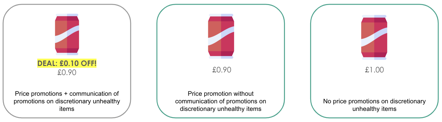
* figures above are illustrative examples
In this study, we found no significant difference between study conditions for total calories (our primary outcome) in the hypothetical order, and no significant difference between study conditions for most of our secondary and exploratory outcomes, including proportion of calories in basket coming from discretionary less healthy foods, the average calorie density of selected products, and the price of the hypothetical order. All three policy options explored in this study received positive net support from the public (ie, more support than opposition). However, the level of support differed significantly between the conditions: allowing discounts and communication of discounts on discretionary less healthy foods (ie, the status quo) had 41% net support, allowing discounts of discretionary less healthy food but removing the communication of these discounts had 20% net support, and removing discounts entirely had 4% net support.
Some results of this simulated supermarket study contradict those from real-world evidence. Specifically, in our study we find no impact of removing discounts from less healthy products, while previous real-world research suggests that this effect is relatively well established. This discrepancy raises questions about the extent to which the overall results of our study are likely to be applicable to the real world. In this report we discuss reasons for why simulated environments might represent a promising setting to generate proof-of-concept evidence for some types of health interventions, but might be less conducive to generate valuable evidence for other policies, such as price-based interventions. In general, we suggest that simulated studies are better suited to study (i) interventions which aim to change behaviour through automatic mechanisms (eg, pre-selecting products by default) and/or (ii) interventions that aim to increase people's comprehension of a given topic rather than eliciting behaviour change (eg, interventions aimed at increasing understanding of healthy eating guidelines). Due to the uncertainty about the real-world applicability of the results, we caution against making policy recommendations solely based on this study.
Introduction
Approximately 63% of adults in the UK are living with overweight or obesity . These conditions are associated with adverse health outcomes including cardiovascular disease, type 2 diabetes, and some forms of cancer. Research suggests that obesity is partly the result of modern food environments (ie, the settings in which people make food selections), which make it increasingly difficult for people to consume healthy foods and to keep within recommended levels of energy intake .
Price promotions on food and drink items represent a key aspect of these modern food environments. There is good evidence that price promotions significantly affect the types and quantity of food selected and that they tend to work particularly well at increasing the purchase of less healthy products . A Public Health England analysis of UK household purchasing data, found that 22% of food and drink purchases could be considered as incremental purchases resulting from price promotions. Revoredo-Giha et al. (2018) found that price promotions increased spending more for less healthy categories (eg, confectionery 10%, sugar and preserves 8%, and soft drinks 6%) than for healthier categories (eg, meats and fish 5%, fruits and vegetables 5%, grains 3%, and dairy 2%) . Nakamura et al. (2015) found that promotions on healthier foods led to a sales uplift of 19.6% and that promotions on less healthy foods led to an uplift of 35% . In addition, research suggests that price promotions are disproportionately applied to less healthy discretionary foods than on healthier products. For example, food and drinks with higher sugar content are more likely to be promoted compared to products with less sugar and in 2020 crisps and snacks were the most purchased items on promotion in Scotland .
As such, most price promotions in the UK are not currently helping families to afford healthy and nutritious foods. Instead, they are mostly designed to nudge consumers into purchasing more unhealthy discretionary products that are high in fat, sugar, and salt (HFSS). In fact, people who buy a large proportion of their foods and drinks on promotion tend to purchase around a fifth more HFSS foods and are more likely to be classified as living with overweight or obesity .
These data have important public health implications in the UK context, where three in ten food and drink items selected are purchased on promotion . To help address this public health challenge, the Scottish Government committed to introduce legislation to restrict promotions on discretionary HFSS products in its 'Programme For Government 2022 to 2023' and consulted on the policy option of restricting Temporary Price Reductions (TPRs) on discretionary less healthy foods . The aim of this policy would be to ensure that consumers are not actively nudged into spending more money on unhealthy foods. However, this policy may still receive significant resistance, as it might be framed and perceived as exacerbating challenges related to rising costs of living.
It is therefore important to explore alternative policy options that could be simpler and more acceptable, yet remain effective at reducing purchases of less healthy discretionary foods. One such alternative – that is the subject of this research – could be to allow industry to continue using temporary price promotions on discretionary HFSS foods but to restrict the communication of these promotions to consumers, ie, any indication on signage or packaging that alerts the consumer to a deal or reduced price (see illustrative example in Treatment 1, Figure 1). This policy was previously consulted on in 2018 in Scotland but received minimal feedback from respondents. To the best of our knowledge there is very limited existing literature looking at the effect of exclusively removing the communication of a discount on less healthy food products, without removing the discount itself.
Figure 1: Illustrative explanation of the business as usual application of temporary price promotion on discretionary HFSS items, and different health policy options
* figures above are illustrative examples
In this project, we investigated the potential impact of removing the communication of temporary price reductions on discretionary HFSS items, on food purchasing behaviour. We also investigated the effect of removing the temporary price reduction entirely. This study was conducted in a simulated online supermarket to generate primary empirical proof-of-concept evidence.
The current study
The full methodology for this study has been pre-registered on the Open Science Framework. In brief, we conducted a three-arm randomised controlled trial with a nationally representative sample of UK adults. Participants were asked to do a hypothetical food order using a simulated online supermarket and were randomly allocated to complete this task in one of three versions of the supermarket:
- Control condition - business as usual: a simulated online supermarket featuring price promotions on discretionary less healthy (ie, HFSS) items and communication of these discounts.
- Treatment 1 condition - discounts with no communication: a simulated online supermarket featuring discounts on discretionary less healthy items, but no communication on these discounts (eg, removal of stickers saying '£X off').
- Treatment 2 condition - no discounts: a simulated online supermarket with no discounts on discretionary less healthy products.
The study aimed to answer five research questions:
- RQ1: Impact of interventions on calorie purchases. How does the removal of discounts on discretionary HFSS items, or the removal of communications of these discounts, affect total calories purchased in a simulated supermarket platform?
- RQ2: Impact of interventions on calorie purchases among subgroups. How does the removal of discounts or the removal of communications of discounts on discretionary HFSS items affect total calories purchased in a simulated supermarket platform among people of different income, BMI and food shopping responsibility?
- RQ3: Impact of interventions on basket price. How does the removal of discounts or the removal of communications of discounts on discretionary HFSS items affect the basket price?
- RQ4: Public support for introduction of intervention. What is the level of public support for the business as usual, for restrictions of discounts on discretionary HFSS products, and for the removal of communication of discounts of discretionary HFSS items?
- RQ5: Interventions' mechanisms of action. Through which mechanisms do discounts and communications of discounts work (eg, increase the number of items purchased; increase energy density of items selected; increase proportion of HFSS)?
Methods
Trial design
The trial was a three-arm randomised controlled trial, with equal randomisation to each trial arm.
Participants
This study recruited a nationally representative sample of adults within the UK from 3 October 2023 to 21 November 2023. The study was closed when the pre-specified sample size of N = 9,000 had been recruited. Participants were sampled using age, gender, income, location, and BMI quotas in order to resemble the demographic distribution of the general UK population. Participants were recruited through the online panel aggregator Lucid. Upon completion of the survey, participants were given a small financial reward for their time through the panel aggregator. Upon entering the study, participants responded to an attention check designed to ensure that they were reading and paying attention to the questions asked. Participants were excluded if they failed the attention check.
Study procedure
Once recruited, participants were directed to the BIT's online experiment platform, Predictiv. On Predictiv, they completed the attention check, answered demographic questions, and were instructed to conduct a hypothetical food order for their household for two days using a simulated online supermarket. Participants were instructed to imagine that they were doing their typical grocery shop and to choose foods and drinks that they and their household would want to eat and that they would be willing to pay for. Participants were permitted to spend however much they chose. To ensure participants understood this task, they had to accurately answer three task-comprehension questions in order to be given access to the simulated supermarket.
Participants were then individually randomised to conduct the hypothetical shopping task in one of three different versions of the University of Oxford's Woods simulated supermarket: the control version, treatment 1, or treatment 2 (see descriptions in the 'interventions' section below). The simulated online supermarket platform for all three conditions was developed by Cauldron, UK and hosted by the University of Oxford. The platform was developed to emulate a real online supermarket, and the site is populated with approximately 9,000 supermarket products that were available for purchase in May 2022. The products are taken from foodDB, a database of food and drinks, which are available for purchase online from six leading UK supermarket retailers. The simulated supermarket was designed to resemble the user experience of a typical online supermarket page, and featured the following interactive interfaces:
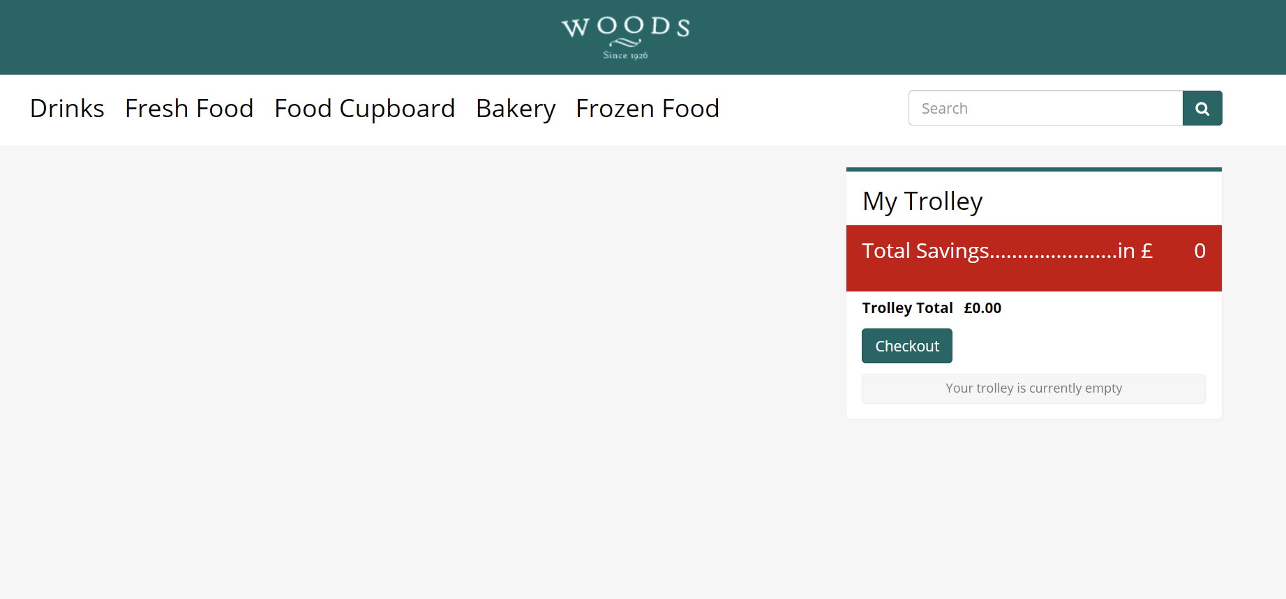
1. Landing page.
Participants started on a landing page with no products displayed and an empty basket. Food categories and the search function are available at the top.
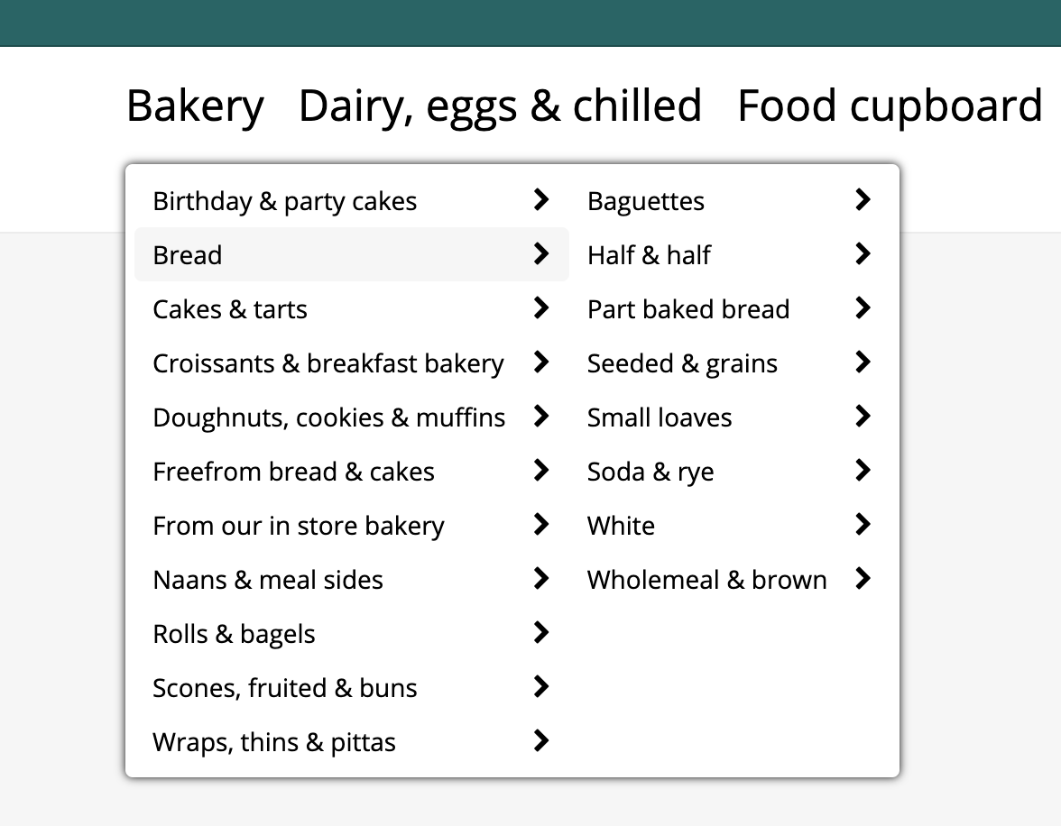
2. Product categories.
Each product category across the top opened up into two levels of sub-categories. Once the participant selected the sub-category, they were taken to the product selection page. Participants could also use the search bar to find products.
3. Product selection page.
On this page, participants were able to select which items they wished to add to their basket, and how many. Products were displayed with the name of the product, its size, the product image, its price and any promotion, as a sticker indicating how much the product had been reduced by.
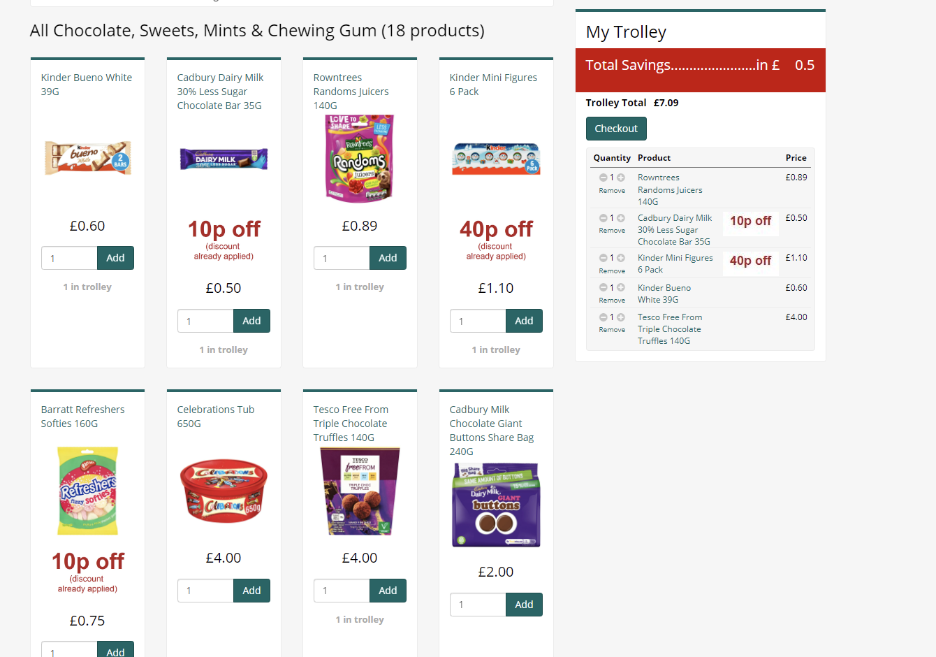
4. My trolley.
In the bottom right corner of the page, participants were able to see their running shopping basket, a running total of the basket price, and a running summary of savings from discounted products. Participants had the option to change the quantity of each product or remove products entirely.
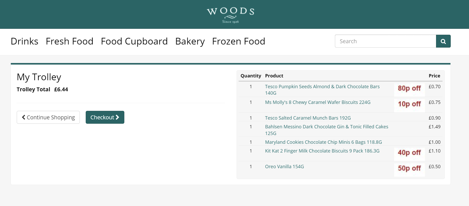
4. Checkout.
At checkout participants were shown the total price of their shop, the products they purchased, and their corresponding quantities and prices. Stickers indicating how much each product has been discounted were displayed.
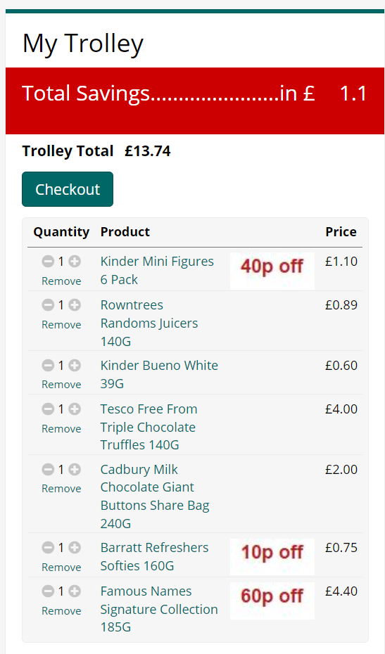
5. Confirmation message. The system prompted users to confirm whether or not they had finished shopping. If the participant selected "No - go back" they were taken back to the checkout page. If they selected "Yes I'm finished", this ended the task and the participant was redirected back to the Predicitv platform. To mitigate the risks of participants not engaging realistically with the simulated supermarket, participants were not able to 'check out' their basket if it had less than two items in it.

Once participants completed the hypothetical food order they were redirected to Predictiv to complete final survey questions.
Interventions
All participants completed the task described above. However they were randomly allocated to complete this task using one of three different versions of the simulated online supermarket. These three versions exclusively differed in (1) whether price promotions were applied on discretionary products high in fat, sugar, and salt or not and (2) whether these price reductions were communicated to consumers through a sticker or not:
- Control condition - business as usual: a simulated online supermarket featuring price promotions on discretionary less healthy (i.e, HFSS) items and communication of these discounts. The number of products discounted and the size of these discounts were broadly representative of a real UK online supermarket. All participants saw the same products discounted.
- Treatment 1 condition - discounts with no communication: a simulated online supermarket featuring discounts on discretionary less healthy (ie, HFSS) items, but no communication on these discounts (eg, removal of stickers saying '£X off').
- Treatment 2 condition - no discounts: a simulated online supermarket with no discounts on discretionary less healthy (ie, HFSS) items.
|
Control |
TR1 (discounts with no comms) |
TR2 (no discounts) |
| Selected HFSS |
Discounted and communicated (random sample of products) |
Discounted but not communicated (random sample of products) |
Not discounted |
| Non-HFSS |
Discounted and communicated (random sample of products) |
Discounted and communicated (random sample of products) |
Discounted and communicated (random sample of products) |
Price promotions and communication of price promotions on non-HFSS items were included and were identical across the three study conditions. HFSS items, as referred to in this protocol, are items which both reach the Nutrient Profiling Model score cut-off point for HFSS and are defined as discretionary by the UK government and are therefore included within the scope of UK regulations on HFSS. See Appendix 1 for more details.
Outcomes
Primary outcome
The primary outcome of this trial is the total number of calories in participants' baskets at checkout. This was calculated from data automatically registered by the simulated online supermarket platform.
Secondary outcomes
There are two secondary outcomes:
Secondary outcome 1: Total price of participants' baskets at checkout. This was calculated from data automatically collected by the simulated supermarket platform.
Secondary outcome 2: Support for promotion restrictions. This was measured through a survey. After completion of the task, participants were asked to indicate their support for the intervention they had been assigned to. Scores range from one (strongly oppose) to five (strongly support).
Exploratory outcomes
There are three exploratory outcomes, all calculated from data that was automatically collected by the simulated online supermarket:
Exploratory outcome 1: Number of items selected in basket at checkout.
Exploratory outcome 2: Proportion of calories in basket from discretionary HFSS items. This is the total calorie content of HFSS items selected divided by total calories of all items in the basket.
Exploratory outcome 3: Average calorie density of basket at checkout. This is the total number of calories divided by the total weight of participants' baskets.
Sample size
We stopped recruitment once we had complete data for 9,004 participants out of the target sample size of 9,000. Based on the target sample of 9,000 participants across three arms, we were powered to detect an effect size of 244 calories (d = 0.054), with a standard deviation estimated at 4,500 calories, 80% power, 5% significance level, and correction for three comparisons. More details about the power calculation can be found in Appendix 3.
Statistical methods
Analytic approach
Prior to analysis, participants meeting a range of exclusion criteria were excluded from the dataset. For example, we excluded participants who had the same participant identifiers, IP addresses, or browser cookies as a previous participant (as these represent data points likely coming from the same person). The full list of exclusion criteria is reported in Appendix 3. There were missing data on education (N = 1,227) and IMD (N = 71) due to errors in the data collection. Multiple imputation was used as the main technique to deal with this missing data. However, to check the robustness of the findings against alternative assumptions, complete case analysis and missing indicator models were also conducted for the primary, secondary, exploratory, and subgroup analyses. More information about this procedure can be found in Appendix 4, and full model results for all methods are reported in Appendix 7.
Covariates
All analyses were adjusted for a range of possible confounding variables. These were gender, age, household income, region of the UK, education, BMI, ethnicity, urbanicity, supermarket shopping frequency, food shopping responsibility, number of people considered in food shop, Index of Multiple Deprivation decile, time of order completion, and day of week of order completion. Full details on how covariates were measured and operationalised can be found in Appendix 5.
Primary outcome analysis
The primary outcome is total calories in the basket. We ran the following Gamma model to estimate the effects of the interventions on total energy ordered by participants in the simulated shopping task:
Total_kcals<sub>i</sub> ~ Gamma(θ, k); log(θ) = α + β + AΓ + ε<sub>i</sub>
- Total_kcalsi is the total calories in the basket of participant i at checkout, and is a positive continuous variable bounded above 0.
- Ti is a factor variable corresponding to the intervention assignment of participant i.
- β refers to the vector of key treatment coefficients.
- A refers to the vector of covariates specified in Table A2 (Appendix 5); Γ refers to the corresponding vector of covariate coefficients.
We estimated heteroskedasticity-robust HC3 standard errors for treatment coefficients. The reported significance of the p-values is after adjusting for three comparisons using the Benjamini-Hochberg step-up procedure to maintain an overall 5% false-discovery rate for the primary analyses.
Secondary and exploratory analysis
We used regression models for the secondary and exploratory outcomes using the same set of covariates. Ordinary least squares regression was used for support of policy interventions, the proportion of basket that is HFSS, and the calorie density of the basket. A Gamma model was used for the total price of participants' baskets. A Poisson model was used for the number of items selected in the basket at checkout. More detailed model specification can be found in Appendix 6.
The secondary outcome analysis was adjusted for six comparisons. The exploratory analysis was not adjusted for multiple comparisons.
Subgroup analysis
We conducted subgroup analyses to look at whether our interventions for our primary outcome (total calories in basket) led to different outcomes for following subgroups of interest:
- Income (bottom quartile <£20k, top quartile >£60k)
- BMI category (People living with overweight/obesity vs not)
- Whether participant makes food shopping decisions ('Yes, all' or ‘Yes, most' vs 'Yes, some' or 'No')
This was conducted using a Gamma model similar to the primary outcome model, but with interaction terms added for the interventions and the subgroups of interest.
Results
Participant flow
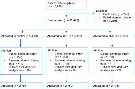
We assessed 15,978 participants for eligibility, randomised 12,423 participants to the three study groups, and analysed data for 8,361 participants.
Figure 2: Participant flow
Baseline data
The demographics of the sample are shown in Table 1 below and were well balanced across study groups.
Table 1: Demographics of each treatment group
| Demographic Category |
Demographic |
Control (n = 2,787) |
Treatment 1 (n = 2,780) |
Treatment 2 (n = 2,794) |
| Age |
Mean (SD) |
42 (15) |
42 (15) |
42 (15) |
| % Female |
|
56% |
55% |
54% |
| Income |
< £20,000 |
25% |
25% |
26% |
|
£20,000-£39,999 |
34% |
31% |
33% |
|
£40,000-£59,999 |
22% |
23% |
23% |
|
≥ £60,000 |
19% |
21% |
19% |
| Location |
South and East |
30% |
30% |
29% |
|
North |
27% |
26% |
26% |
|
Midlands |
18% |
18% |
18% |
|
London |
12% |
13% |
13% |
|
Scotland, NI, Wales |
13% |
14% |
14% |
| BMI |
Mean (SD) |
26.12 (6.53) |
26.29 (6.82) |
26.31 (6.89) |
| Ethnicity |
White UK |
82% |
81% |
82% |
|
Asian or Asian British |
6% |
6% |
6% |
|
Black |
4% |
6% |
5% |
|
White Other |
5% |
5% |
4% |
|
Mixed |
2% |
2% |
2% |
|
Other |
1% |
1% |
1% |
| Education |
Less than high school |
4% |
3% |
4% |
|
High school completed |
21% |
20% |
21% |
|
University degree |
37% |
37% |
39% |
|
None of the above |
23% |
25% |
22% |
|
Missing |
15% |
15% |
14% |
| Index of Multiple Deprivation |
1st decile |
6% |
6% |
6% |
|
2nd decile |
7% |
6% |
6% |
|
3rd decile |
7% |
9% |
8% |
|
4th decile |
20% |
20% |
18% |
|
5th decile |
13% |
14% |
16% |
|
6th decile |
11% |
12% |
11% |
|
7th decile |
11% |
10% |
11% |
|
8th decile |
8% |
8% |
7% |
|
9th decile |
10% |
10% |
9% |
|
10th decile |
6% |
5% |
5% |
| Missing |
|
1% |
1% |
1% |
| Number of people in household |
|
|
|
|
|
1 |
14% |
15% |
16% |
|
2 |
34% |
32% |
32% |
|
3 |
23% |
22% |
21% |
|
>3 |
29% |
31% |
31% |
| Responsible for shopping |
|
|
|
|
|
Yes |
86% |
86% |
86% |
|
No |
14% |
14% |
14% |
Note: Percentages may not sum to 100 due to rounding.
Outcomes and estimation
Compared to the control condition, no intervention led to significant changes in the total calories ordered, the price of the basket, the proportion of basket that is HFSS items, or the calorie density of the basket. There was also no difference in these outcomes between the two interventions. All three policy options explored in this study received positive net support from the public (ie, more support than opposition). However, the level of support differed significantly between the policy options: both treatment groups showed significantly lower ratings of support for their respective policies than the control group, and the removal of discount was significantly less supported than the removal of communication of discounts on discretionary less healthy products. Below we present the results from our main model (Multiple Imputation). Results were consistent across all three models (Multiple Imputation, Missing Indicator, Complete Case), supporting their robustness. Full outputs for all models are in Appendix 7.
Primary outcome
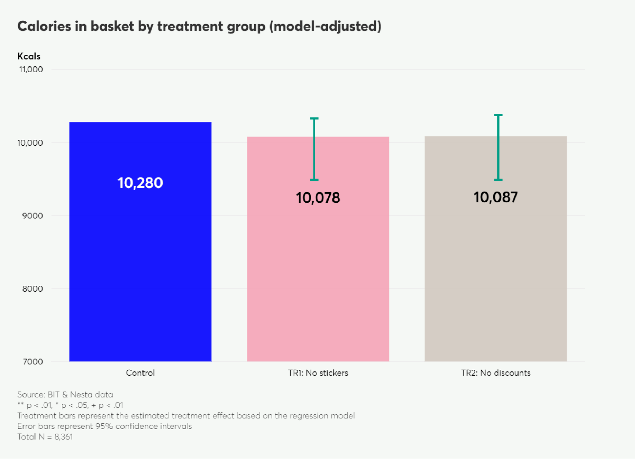
There was no statistically significant difference in the total calories of the final basket across the three study conditions, although – directionally – participants in the intervention groups purchased fewer calories than those in the control.
- The control group had an average of 10,280 calories in the basket.
- TR1 had an estimated average of 10,078 calories in the basket (effect estimate: -201kcal, 95%CI: -650kcal to +269kcal, p=.395).
- TR2 had an estimated average of 10,087 calories in the basket (effect estimate: -193kcal, 95%CI: -648 to +285kcal, p=.423).
- TR2 was not significantly different from TR1 (effect estimate: -9kcal, 95%CI: -449kcal to + 489kcal, p = .97).
Figure 3 shows the raw control group mean and the estimated treatment effect in the treatment groups according to the regression model.
Figure 3: Model-adjusted calories in basket by treatment group
Secondary outcomes
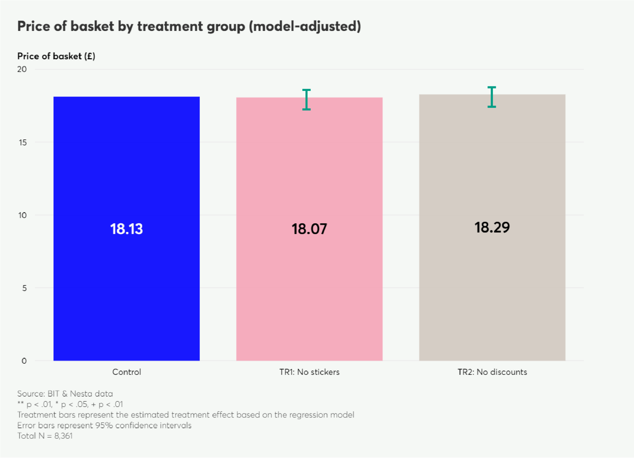
There was no statistically significant difference in the total price of the basket across the three study conditions.
- The control group had an average total price of £18.13.
- TR1 had an average estimated price of £18.07 (effect estimate: -£0.05, 95%CI: -£0.68 to +£0.59, p=.867).
- TR2 had an average estimated price of £18.29 (effect estimate: £0.16, 95%CI: -£0.47 to +£0.82, p=.622).
- TR2 was also not significantly different from TR1 (effect estimate: £0.22, 95%CI: -£0.42 to +£0.88, p=.509).
Figure 4 shows the raw control group mean and the estimated treatment effect on both treatment groups according to the regression model.
Figure 4: Model-adjusted price of basket by treatment group
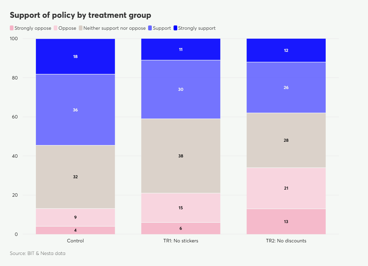
All three policy options explored in this study received positive net support from the public (ie, more support than opposition). However, the level of net support differed significantly between the different policy options:
- When asked to rate their support for the policy that they were exposed to, the control group had a net support (all support - all opposition) of 41%.
- TR1 had a net support of 20%.
- TR2 had a net support of 4%.
Figure 5 below shows the raw proportions of each level of support (Strongly support; Support; Neither support nor oppose; Oppose; Strongly oppose) by treatment group. There was a significant reduction in average support for TR1 compared to control (estimated effect: -0.28, 95%CI: -0.34 to -0.23, p <.001), TR2 compared to control (estimated effect: -0.51, 95%CI: -0.56 to -0.45, p <.001), and TR2 compared to TR1 (estimated effect: -0.22, 95%CI: -0.28 to -0.17, p <.001).
Figure 5: Support of policy by treatment group
Exploratory outcomes
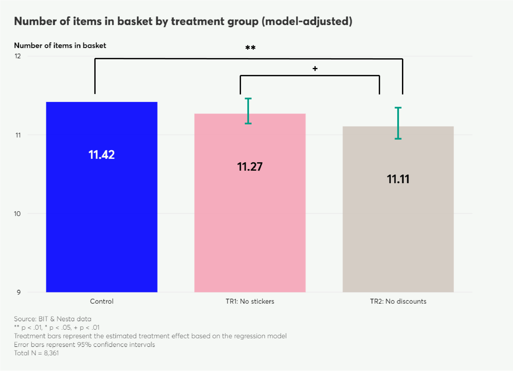
TR2 (removal of discounts) significantly reduced the number of items purchased compared to the control group, with an estimated treatment effect of -2% (95%CL: -4% to -1%, p = .003). TR1 did not differ significantly from either the control group (estimated effect: -1%, 95%CI: -3% to +1%, p = .203) or TR2 (estimated effect: -1%, 95%CI: -3% to 0% ,p = .081) on the number of items in the basket.
Figure 6 shows the raw control group mean and the estimated treatment effect on both treatment groups according to the regression model.
Figure 6: Model-adjusted number of items in basket by treatment group
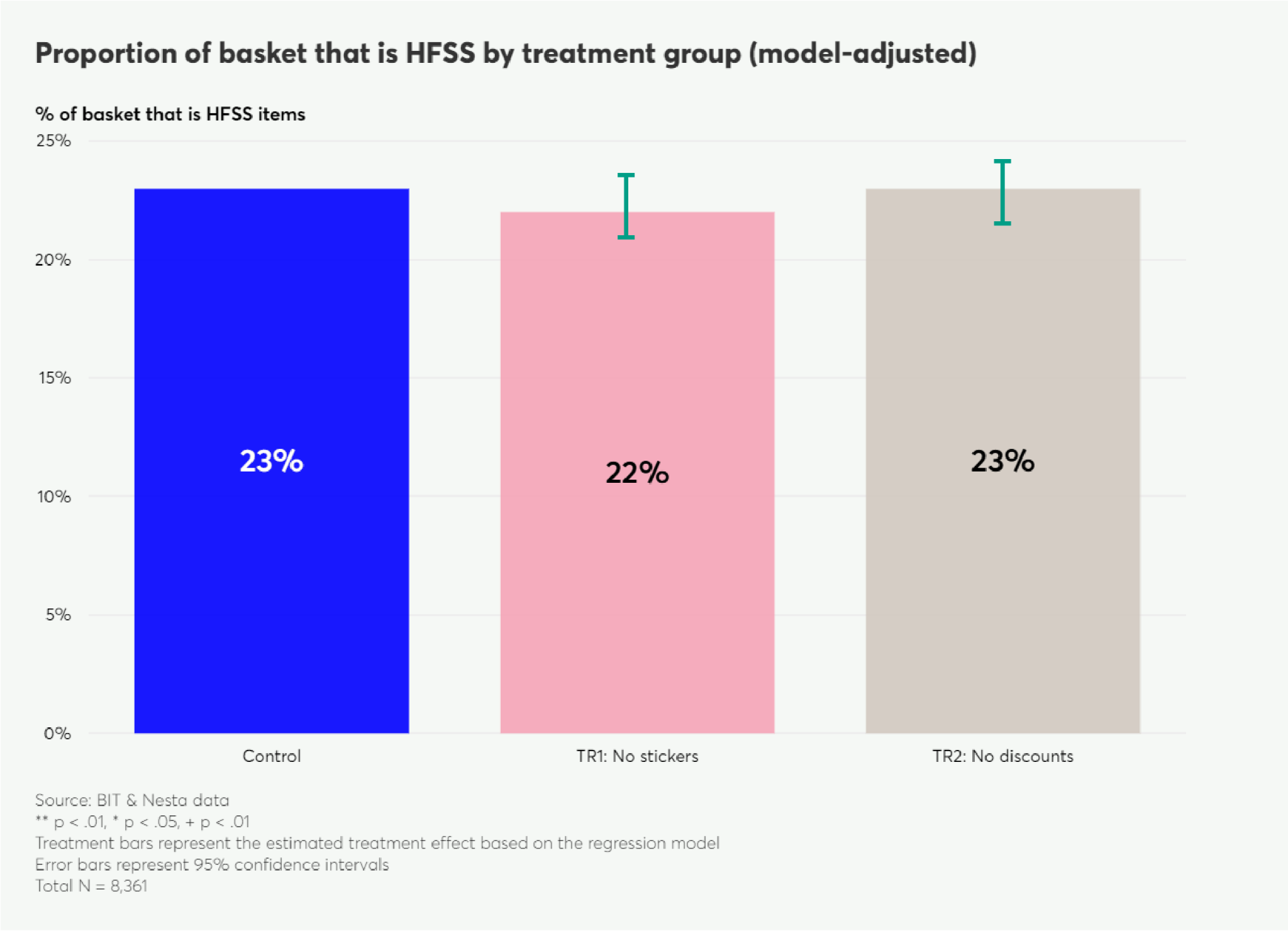
There was no significant difference in the proportion of the basket that is made up of HFSS items across the three study conditions.
- In the control group, 23% of the basket was HFSS items.
- In TR1, the proportion was 22% (estimated effect: -1pp ; 95%CI: -2pp to 0pp, p=.188).
- In TR2, the proportion was 23% (estimated effect: 0pp; 95%CI: -2pp to +1pp, p= .599).
TR2 was not significantly different than TR1 (estimated effect: 1pp, 95%CI: -1pp, +2pp, p=.428). Figure 7 shows the raw control group mean and the estimated treatment effect on both treatment groups according to the regression model.
Figure 7: Model-adjusted proportion of basket that is HFSS by treatment group
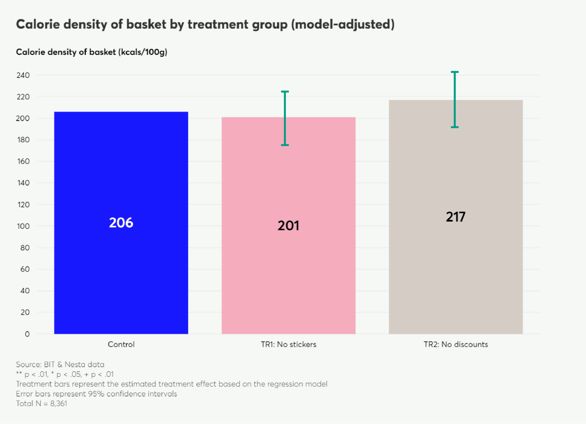
There were no significant effects of treatment on the calorie density of the basket (kcals/100g).
- In the control group, the calorie density was 206 kcals/100g.
- In TR1, the calorie density was 201 kcals/100g (- 5 kcals/100g, 95%CI: -30 to +20, p = .695).
- In TR2, the calorie density was 217 kcals/100g (+12 kcals/100, 95%CI: -13 to +36, p = .355).
TR2 was not significantly different from TR1 (estimated effect: 17, 95%CI: -8 to +41, p = .187). Figure 8 shows the raw control group mean and the estimated treatment effect on both treatment groups according to the regression model.
Figure 8: Model-adjusted calorie density by treatment group
Subgroup analysis
An exploratory subgroup analysis was conducted to see whether the effects of treatment on the calories in the basket varied based on BMI, income, and responsibility for household shopping. For income and shopping responsibility, there were no significant interactions. The non-significant effect on calorie purchases of TR1 or TR2 compared to control did not differ for participants living with overweight/obesity compared to those not living with overweight/obesity (p = .375, p = .094, respectively). When comparing TR2 to TR1, there was a significant interaction between treatment and BMI such that participants living with overweight and obesity purchased more calories in all study conditions, but this difference was significantly more pronounced in TR2 compared to TR1 (p = .011).
Additional analysis
For every pound increase in experimental spend, self-reported spend increased by an average of £0.26 (95%CI: £0.24 to £0.28, p < .001). The adjusted R squared of the linear regression is 0.07, indicating that experimental spend only explains 7% of the variance in self-reported actual spend.
Discussion
The aim of this study was to test how purchasing behaviour is affected by either removing price promotions on discretionary less healthy food and drinks, or removing any communication of the price promotions of discretionary less healthy food and drinks, without removing the actual discounts. Our study found no significant difference between the control group and the two treatment groups for the number of calories ordered, the price of the shopping basket, the proportion of the basket that is HFSS, and the average calorie density of the items selected. We did find a significant decrease in the number of items purchased in the condition where discounts were removed. All policy options explored in this study received net public support but there were significant differences between arms: net support for the control condition, ie, allowing discounts on HFSS items and communicating these, was 41%. Removing communications of discounts, without removing the discounts themselves, received 20% net support and removing discounts entirely 4%. This suggests that the two policies tested are supported by the majority of people, but they are not as well supported as the current status quo, and removing communication from discounts on discretionary HFSS products is more supported than completely removing discounts from these products.
This study had a number of strengths. We had a large nationally representative sample size, with 8,361 participants completing the task. The simulated store closely resembled the target setting, ie, online grocery stores. The foods were drawn from a database that was reflective of product options and prices from the top six UK supermarkets. The number of discounts and magnitude of discounts were also based on actual data from a UK supermarket (see Appendix 2). Additionally, 79% of the sample reported shopping online at least once a month, indicating that for a large majority of the sample, the behaviour of ordering groceries from an online retailer was similar to their regular grocery shopping habits.
However, some key findings in this study are not in line with the existing literature. Multiple previous studies find an effect of discounts on purchasing behaviour of foods and drinks. Our finding that removing discounts on HFSS items did not lead to a statistically significant change in calories contradicts previous research. There is
very limited existing literature on the effect of only removing the communication of discounts (ie, treatment group 1) to compare our results to. However, the fact that removing price promotions did not lead to a well-established behavioural effect suggests that the wider external validity of this project needs to be taken with caution. Further research needs to be conducted in the real world before making any strong policy recommendations about the investigated policy options.
We propose three methodological reasons why our results may differ to the existing literature and explore these in turn below:
- Simulated experiments may not be appropriate to study price interventions which may explain the differences between our results and those from non-simulated studies.
- Methodological differences between previous simulated trials and ours may explain the difference between our results and those from other simulated trials.
- The analysis of our study may have been underpowered.
Simulated studies always feature a range of limitations in regard to their generalisability to the real world. We believe this might be particularly so for price-based interventions, such as the ones explored in this study. The consequences of the real-life behaviour of shopping for groceries include spending money and having to consume the foods, both of which are absent in the simulated shopping environment.
The removal of financial consequences is particularly challenging for this study. Price-based interventions rely on the price of the items being a driving factor of decision-making, as they assume that changing the price will lead to changes in decision-making. A simulated environment in which no real money is spent removes the incentive to consider price and limit the overall price of the basket. The suggestion that people may not have considered product prices as they would otherwise do in the real world is supported by our data, as there was only a small association between people's self-reported real-life spend on groceries and how much they spent in the task.
Studies investigating the impact of price promotions conducted in real-world environments – ie, where participants spend money and receive food and drink items – have found price promotions to be an important determinant of purchasing behaviour.
Several studies using demand models to analyse UK household purchasing data have found that price promotions are associated with significant increases in the purchasing of promoted products,,,. Also, a systematic review of RCTs found that eight out of the nine studies of price promotions in real stores found an effect of promotions on purchasing behaviour. The effects of the price-based interventions included in the review were not combined into a single effect estimate, but some of the effects were large: in one trial the percentage of participants who consumed sufficient amounts of fruit and vegetables increased from 42.5% at baseline to 61.3% at 6 months in the discount groups (p = 0.03). For the non-discount groups, these percentages were 52.7% and 52.5%, respectively (p = 0.80). The fact that some of our key results do not align with those from real-world studies suggests that the use of a simulated environment may not have been an effective approach to generate proof-of-concept evidence for our specific research questions. Other types of interventions may be more appropriate to test in simulated environments. Specifically, we hypothesise that:
- Interventions that work through automatic mechanisms, such as framing, defaults, or repositioning, may still be suitable to be tested in a simulated environment. Even in the real world, such interventions do not rely on a conscious appraisal of the consequences of one's behaviour (eg, trying to avoid spending more money), so the automatic reactions that take place in a simulated environment are likely to replicate in the real world (albeit likely with smaller effect sizes).
- Interventions that aim to increase people's comprehension of a given topic (eg, interventions and trials testing how to increase people's understanding of healthy eating guidelines) are also more appropriate for simulated experiments: if a participant understands a guideline better in a simulated environment it is likely that they would also understand this guideline better in the real world.
Methodological differences between this study and previous simulated trials
In the previous section, we argue that one reason why our findings might diverge from real-world research, is because we tested price-based interventions in a simulated supermarket where participants were not asked to spend real money. However, previous studies of price-based interventions conducted in simulated shopping environments did generate results which are in line with real-world experiments: six experiments included in a 2018 systematic review report finding statistically significant effects of price interventions on absolute measures of purchasing behaviour in simulated environments. Similarly, a 2023 study by Luick et al., which used the same simulated environment as in this study, also found an effect on price promotions on purchasing.
One explanation for this difference is that previous studies included budgets for the simulated shopping task, ie, participants were told how much money they should spend in the hypothetical shopping task, which was not the case in our study. There are several reasons why setting a budget may explain the discrepancy between our results and those of previous simulated studies:
- First, setting a budget may make prices more salient to participants: in a simulated context, where money is not spent and items are not received, there is little incentive to pay attention to price. By setting a budget these studies might have raised the salience of price in the simulated context.
- The second – and more problematic – reason why setting a budget may impact results is that a budget may create a ceiling effect of sorts: participants in a treatment condition where prices for unhealthy items are lower (due to price promotions) are simply able to add more of these items to their baskets within the pre-specified budget. Conversely, participants in conditions where price promotions are removed, can add fewer of these items within the pre-specified budget. This could artificially enhance the extent to which removing price promotions is found to influence purchasing behaviours in simulated environments.
For future research on price-based interventions promoting healthier food purchasing behaviour we recommend prioritising real-world trials over stimulated studies. If a simulation is selected nonetheless, then efforts should be made to replicate the real-world consequences. A possible set up for a simulated study that goes some way towards addressing the limitations identified above could be the following:
| Feature of study design | Rationale |----------|----------|
| 1. Provide a budget to participants. | Having a budget ensures that participants' shopping behaviour represents a broadly realistic amount of food purchasing for the set task. To increase the relevance of this budget, shoppers could be asked to self-select a |----------|----------|
| 2. Ensure that the budget is indicative rather than fixed. |----------|----------|
1Provide a budget to participants.
2Ensure that the budget is indicative rather than fixed.
3Operationalise the outcome as the relative proportion of the basket made up by the targeted foods, rather than focussing on absolute amounts of the target foods purchased.
Power of the study
A third reason which may explain the difference between our results and those in previous studies, both simulated and real-world trials, is that our study may have been underpowered. If the assumptions of our power calculation were met, then we would have been powered to detect effects of approximately 240 kcals, which is conservative compared to previous research which has shown effects of 552 kcals, or 10% of the total basket. The observed standard error was more than double the assumed standard adding noise to our estimation. Under these circumstances, only an effect size upwards of 727 kcals per shopping trip would have been picked up 80% of the time.
Conclusion and future research
This study investigated the impact of removing the communication of price promotions and the effect of removing price promotions entirely on discretionary products high in fat, sugar, and salt (HFSS) in a simulated online shopping environment. The study found no significant effect of these interventions on our primary outcome, calories ordered, and most of the secondary and exploratory outcomes. Some results of this simulated supermarket study contradict those from real-world evidence. Specifically, in our study we find no impact of removing discounts from less healthy products, while previous real-world research suggests that this effect is relatively well established. This discrepancy raises questions about the extent to which the overall results of our study are likely to be applicable to the real world. Due to this, we caution against making policy recommendations solely based on this study.
As identified in Watt et al (2020), more studies are required to understand the extent to which restricting promotions on discretionary less healthy products may reduce consumption of less healthy food products. Based on this study, we would recommend testing these price-based interventions through real-world trials, rather than attempting to generate proof-of-concept evidence via a simulated environment. Future trials of health promoting interventions should carefully consider whether the research question is appropriate for a simulated experiment, by considering whether the intervention acts through automatic or conscious behavioural mechanisms, whether the real-world incentives can be mimicked in the simulated environment, whether the outcome is a change in behaviour or change comprehension, and the importance of contextual factors that are difficult to replicate in simulated environments, such as mood. In particular, we suggest that simulated studies are better suited to study (i) interventions which aim to change behaviour through automatic mechanisms (eg, pre-selecting products by default) or (ii) interventions that aim to increase people's comprehension of a given topic rather than modifying their behaviour (eg, interventions aimed at increasing understanding of healthy eating guidelines).
Appendix 1- Nutrient Profiling Model scores and High Fat, Salt, and Sugar classification
Nutrient Profiling Model (NPM) scoring:
- Scores were calculated according to technical guidance set out by the Department of Health in 2011.
- Fruit, vegetable and nut (FVN) scores were not available at a product level. Therefore, these were allocated at a product category level by Nesta and then these scores were reviewed and adjusted by Oxford University. Where we felt that the category allocation was too broad, we used keyword matching within categories to allocate FVN scores to products.
HFSS classification:
- Each product category was allocated as either in-scope or out-of-scope of HFSS regulations, according to guidance set out by the Department of Health and Social Care.
- Products were classed as HFSS if they were both in-scope of HFSS regulations and reached the threshold NPM scores.
Some limitations of our NPM/HFSS approach include:
- We allocate FVN scores mostly at a product group level, inevitably leading to inaccuracies in NPM scoring.
- Assuming 1 gram = 1 millilitre and not using product-specific gravities to convert from millilitres to grams accurately.
- We do not include reconstitution factors for products which require reconstitution as per HFSS regulations.
Appendix 2 - Calculation of number and size of discounts
In order to make the study as realistic as possible we based the number of products to discount, and the size of these discounts, on purchasing data of a UK online supermarket. Food and drink purchasing data was provided by an international market research company. The analysis was conducted as follows, we:
- kept purchasing data only from a single large online UK supermarket
- kept only unique purchases from this supermarket for each day
- calculated the percentage of products on promotion within each product category (excluding multi-buy and ‘extra free' promotions, due to inability to include these on Woods platform)
- calculated, for products with a discount, the discount sizes as a percentage of total price, and split these discounts into quartiles by frequency of occurrence of the discount sizes
- calculated the mean discount size within each quartile.
To apply these discounts we applied the numbers in the analysis to the Woods platform by:
- taking each category and applying discounts to a random selection of products within each category. The number of products to be discounted was based on the percentage of products identified as discounted within the category in the preceding analysis
- randomly assigned the products to be discounted into four groups within each category. Each of the four groups was then allocated a discount size (as a percentage) corresponding to the four mean discounts per quartile, within each product category, as determined by the preceding analysis
- Calculating discounts in pounds and pence off and rounded to the nearest 10p for all discounts up to £2.50. For products above £2.50 discounts were rounded to the nearest 50p.
Some ways in which this procedure may have led to an over- or under-estimation of the number and size of discounts include:
- The fact that this is purchasing data, therefore, products on discount are likely to be over-represented in the data.
- To reduce this we only used data on unique purchases each day, however, there is likely to still be some over-estimation of the number of products on discount.
- We excluded multi-buy and 'extra free' discounts from our analysis of the number of promotions.
- 6.9% of products in our dataset were on multi-buy discount.
- 0.04% of products in our dataset had an 'extra free' discount.
- This will have led to an under-estimation of the number of products on discount.
- The purchasing data top-codes all discounts above £2 to £2+. We treat these discounts as £2.
- 12% of discounts fall into this category.
- This will have led to an under-estimation of the discount sizes for our top quartiles of discounts.
Appendix 3 - Sample size calculation and data cleaning specification
Prior to commencing data collection, a power analysis was conducted based on the following assumptions:
- We expected the average person to order 8,000-10,000 calories for their household for two days. This is based on the average UK household having 2.4 residents and previous work by Nesta shows that the mean amount of calories bought in a supermarket for a person for one day is 1,800 calories.
- In a recent study conducted in Singapore, using a simulated online supermarket where participants were asked to perform a shopping task for themselves for one week with a SGD 50-250 (£30-£150) budget, participants ordered an average of 11,765 calories (sd = 8,270).
- However, we expected there to be a large variance around the mean calorie intake for households. We conducted a power analysis for a range of outcome standard deviations (from 2,000 to 8,000 calories).
- Considering our task is more constrained than the Singapore study task (just two days), we expect an outcome SD to be lower, at ~ 4,500 calories.
Given a sample of 9,000 participants, three trial arms, adjusting for three comparisons (all treatment versions are to be compared against the control and to each other) via the Bonferroni correction, we were powered to detect an effect size of 244 calories (d = 0.054). This assumes an outcome standard deviation of 4,500 calories.
Our power estimates can be considered conservative. In the primary and secondary analysis, we controlled for the false-discovery rate (not the family-wise error rate) using the Benjamini-Hochberg procedure, which is less stringent on p-values than the Bonferroni correction. Covariates were also included, increasing the precision of our estimates and thus our statistical power.
|
Main analysis (primary outcome) |
Secondary outcomes |
| Minimum Detectable Effect Size (MDES) |
Cohen's d = 0.047 (~254 calories) |
Cohen's d = 0.089 |
| Alpha |
0.017 (0.05/3) |
0.008 (0.05/6) |
| Power |
0.80 |
0.80 |
| One-sided or two-sided? |
two-sided |
two-sided |
| Number of participants Intervention arms |
~3000 x2 |
~3000 x2 |
| Control |
~3000 |
~3000 |
| Total |
9000 |
9000 |
| Software used for calculation |
R |
|
Prior to analysis, participants were excluded from the dataset if they met any of the following exclusion criteria:
- Those with duplicated participant identifiers, IP addresses, or browser cookies (as these represent data points likely coming from the same person). Only the first chronological record was kept.
- Those who dropped out from the experiment before completing it. At this stage, we also checked for differential attrition by trial arm, and found no evidence that there was differential attrition.
- Outliers based on the price of the basket per household member. Outliers were defined (post data collection) as those who fell more than 1.5 times the interquartile range below quartile 1 or above 1.5 times the interquartile range above quartile 3. 612 participants were excluded for having values higher than the threshold; no participants were excluded for having values lower than the threshold.
Appendix 4 - Missing data
- Three participants were missing gender data, 26 participants had missing BMI data and five participants were missing data on an outcome measure (proportion of basket that is HFSS items). Due to the small number of cases that were missing data on these measures, listwise deletion was used as it is unlikely to bias the results.
There was a technical error in the collection of education data on the Predicitv platform, so this data was missing for all participants. For 7,134 participants this data was retrieved from the panel provider, leading to 1,227 instances of missing data in the final dataset. Additionally, 71 participants were missing IMD data due to participant errors in inputting the required data (first half of postcode), which meant their postcode was unable to be matched to an IMD decile. As the cause of both sources of missing data was due to errors, we assumed that they are Missing Completely At Random (MCAR). In order to retain data (and therefore statistical power), multiple imputation was chosen to handle the missing data.
The missing data was imputed based on the covariates and endpoints: BMI, age, gender, ethnicity, education, region in the UK, income, urbanicity, treatment, shopping frequency, shopping responsibility, number of people in household, timing of order, day of order, calories ordered, price of order, support for policies, number of items ordered, proportion of order that is HFSS, and the calorie density. Predictive mean matching within the 'mice' R package was used to impute the data. Five imputation datasets were used with 15 iterations each.
Appendix 5 - Covariates
Table A2 lists the covariates that were used in all regression models and their coding. For the missing indication model, the deprivation decile and education variables included an additional dummy variable for missingness.
Table A2: Trial covariates used in the analyses
| Measure | Vector | Definition | Coding |----------|----------|
| Description | Metric | | Measurement period | Baseline | TR1 (no stickers) | TR2 (no discounts) | Difference to Control | (p-value) |
|:----------------|:-----------|:--------------------------------------------------------|:--------------------------|:-------------|:----------------------|:-----------------------|:--------------------------|:----------------------------|
| Price of basket (GBP) | Mean | The average amount of money a customer spends. | Post-treatment (T4-T16) | £18.24 | £18.07 | £18.29 | -£0.16 | (p=0.20) |
| Calorie density of basket (kcal/100g) | Mean | The average calorie content per 100g of products. | Post-treatment (T4-T16) | 210.15 | 216.51 | 201.27 | -8.88 | (p=0.07) |
| HFSS proportion of basket (%) | Mean | The percentage of items in a basket that are HFSS. | Post-treatment (T4-T16) | 22.84 | 22.83 | 22.19 | -0.65 | (p=0.36) |
| Number of items in basket | Mean | The total count of unique products in the basket. | Post-treatment (T4-T16) | 11.42 | 11.27 | 11.11 | -0.31 | (p=0.20) |
| Policy support score (1-5 scale) | Mean | A Likert scale score indicating approval for the policy. | Post-treatment (T16) | 2.54 | 2.24 | 2.03 | -0.51 | (p<0.001) |
Finkelstein, E.A., Ang, F.J.L. & Doble, B. Randomized trial evaluating the effectiveness of within versus across-category front-of-package lower-calorie labelling on food demand. BMC Public Health 20, 312 (2020). https://doi.org/10.1186/s12889-020-8434-1
| Variable | Code | Question/Definition | Categorical Mapping | Variable Name ```
Note: The following footnotes were found on page 47 of the source document and are applicable to the preceding content.

Table A6 below shows the full model results for the exploratory outcome of number of items in the basket. The significance of covariates has not been corrected for multiple comparisons.
Table A6: Full results for number of items in basket. Cells represent the estimated multiplicative effect of each variable, with 95% confidence limits in parentheses.
Outcome: Number of items in basket
| Category |
Multiple Imputation |
Missing Indicator |
Complete Case |
| Other |
-0.13 (-0.41,0.14) |
-0.13 (-0.4,0.15) |
-0.09 (-0.42,0.23) |
| Shopping frequency (reference category is more than once a week) |
|
|
|
| Once a week |
0.01 (-0.07,0.1) |
0.01 (-0.07,0.1) |
-0.01 (-0.1,0.08) |
| A few times a month |
0.03 (-0.08,0.13) |
0.03 (-0.08,0.14) |
-0.02 (-0.14,0.09) |
| Once a month |
0.06 (-0.27,0.39) |
0.06 (-0.27,0.39) |
0.12 (-0.23,0.47) |
| Never |
0.3 (-0.46,1.07) |
0.3 (-0.46,1.06) |
0.33 (-0.48,1.13) |
| Shopping responsibility (reference category is none of it/some of it) |
|
|
|
| Most of it/all of it |
0.09* (0.01,0.16) |
0.09* (0.01,0.16) |
0.07 (-0.01,0.14) |
| Number of people in household (reference category is 1) |
|
|
|
| 2 |
0.05 (-0.03,0.12) |
0.05 (-0.03,0.12) |
0.05 (-0.03,0.13) |
| 3 |
0.06 (-0.02,0.14) |
0.06 (-0.02,0.15) |
0.04 (-0.04,0.13) |
| More than 3 |
0.04 (-0.04,0.12) |
0.04 (-0.04,0.12) |
0.03 (-0.06,0.11) |
| Time of day (reference category is morning) |
|
|
|
| Lunch |
-0.03 (-0.09,0.03) |
-0.03 (-0.09,0.04) |
-0.02 (-0.09,0.05) |
| Dinner |
-0.04 (-0.1,0.02) |
-0.04 (-0.1,0.02) |
-0.05 (-0.11,0.02) |
| Night |
0 (-0.08,0.08) |
0 (-0.08,0.08) |
0.01 (-0.07,0.1) |
| Day of the week (reference category is Monday) |
|
|
|
| Tuesday |
0.03 (-0.05,0.12) |
0.03 (-0.05,0.12) |
0.04 (-0.06,0.13) |
| Wednesday |
0 (-0.1,0.1) |
0 (-0.1,0.09) |
0.02 (-0.08,0.13) |
| Thursday |
0.02 (-0.06,0.1) |
0.02 (-0.06,0.1) |
0.02 (-0.07,0.1) |
| Friday |
-0.03 (-0.13,0.07) |
-0.03 (-0.13,0.07) |
-0.03 (-0.14,0.08) |
| Saturday |
0.07 (-0.06,0.2) |
0.07 (-0.06,0.2) |
0.08 (-0.05,0.22) |
| Sunday |
0.03 (-0.07,0.13) |
0.03 (-0.07,0.13) |
0.04 (-0.06,0.15) |
| Deprivation Decile (reference category is 1) |
|
|
|
| 2 |
0.02 (-0.11,0.16) |
0.11 (-0.03,0.24) |
-0.01 (-0.15,0.13) |
| 3 |
-0.14* (-0.24,-0.03) |
0.12+ (-0.02,0.26) |
-0.13* (-0.25,-0.02) |
| 4 |
0 (-0.08,0.09) |
0.13+ (-0.01,0.28) |
-0.01 (-0.11,0.08) |
| 5 |
-0.03 (-0.11,0.05) |
0.15+ (-0.01,0.3) |
-0.06 (-0.15,0.03) |
| 6 |
0.03 (-0.05,0.11) |
0.15+ (-0.01,0.3) |
0.05 (-0.03,0.14) |
| 7 |
0 (-0.08,0.08) |
0.17* (0.01,0.32) |
-0.03 (-0.11,0.06) |
| 8 |
0.01 (-0.07,0.09) |
0.14+ (-0.02,0.3) |
0.02 (-0.07,0.1) |
| 9 |
-0.01 (-0.08,0.06) |
0.09 (-0.07,0.25) |
-0.01 (-0.08,0.07) |
| 10 |
-0.01 (-0.07,0.06) |
0.05 (-0.12,0.23) |
0.01 (-0.06,0.08) |
| Missing |
NA |
-0.05 (-0.33,0.24) |
NA |
| Education (reference level is less than high school) |
|
|
|
| High school completed |
-0.01 (-0.14,0.12) |
0.01 (-0.13,0.14) |
0.01 (-0.13,0.14) |
| University degree |
0.02 (-0.1,0.15) |
-0.01 (-0.09,0.07) |
0.03 (-0.1,0.16) |
| None of the above |
0.08 (-0.05,0.22) |
0.09* (0.02,0.17) |
0.09 (-0.05,0.22) |
| Missing |
NA |
0.03 (-0.03,0.1) |
NA |
| BMI (reference level is underweight) |
|
|
|
| Healthy weight |
-0.02 (-0.13,0.08) |
-0.03 (-0.13,0.08) |
-0.04 (-0.15,0.07) |
| Living with overweight |
-0.04 (-0.14,0.07) |
-0.04 (-0.14,0.07) |
-0.05 (-0.17,0.06) |
| Living with obese |
-0.1+ (-0.21,0) |
-0.1+ (-0.21,0) |
-0.12* (-0.24,-0.01) |
| Total N |
8,361 |
|
7,073 |
| Control Mean |
11.42 |
|
11.24 |
| Intercept |
4.65** (4.33,4.98) |
4.84** (4.55,5.16) |
4.66** (4.37,4.97) |
| Treatment Group |
|
|
|
| TR1 vs Control |
0.99 (0.97,1.01) |
0.99 (0.98,1.01) |
0.99 (0.97,1) |
| TR2 vs Control |
0.98** (0.96,0.99) |
0.98** (0.96,0.99) |
0.97** (0.96,0.99) |
| TR2 vs TR1 |
0.99+ (0.97,1) |
0.99+ (0.97,1) |
0.99+ (0.97,1) |
| Gender (reference category is Male) |
|
|
|
| Female |
1.22** (1.2,1.24) |
1.22** (1.2,1.24) |
1.22** (1.2,1.24) |
| Other |
1.11* (1.01,1.22) |
1.11* (1.01,1.22) |
1.18** (1.07,1.3) |
| Age (reference category is 18-24) |
|
|
|
| 25-34 |
1.03* (1,1.05) |
1.03* (1,1.05) |
1.02 (0.99,1.05) |
| 35-44 |
1.06** (1.04,1.09) |
1.07** (1.04,1.09) |
1.07** (1.04,1.09) |
| 45-54 |
1.11** (1.08,1.14) |
1.11** (1.08,1.14) |
1.09** (1.06,1.12) |
| 55-64 |
1.27** (1.23,1.3) |
1.27** (1.23,1.3) |
1.26** (1.22,1.29) |
| 65+ |
1.18** (1.14,1.22) |
1.18** (1.14,1.21) |
1.19** (1.15,1.24) |
| Income (reference category is under £20,000) |
|
|
|
| £20,000-£39,999 |
1.01 (1,1.03) |
1.01 (1,1.03) |
1.01 (0.99,1.03) |
| £40,000-£59,999 |
1.03* (1.01,1.05) |
1.03** (1.01,1.05) |
1.02+ (1,1.04) |
| Over £60,000 |
1.06** (1.04,1.08) |
1.06** (1.04,1.08) |
1.04** (1.02,1.07) |
| Location (reference category is London) |
|
|
|
| North |
1.03* (1,1.05) |
1.03* (1,1.05) |
1.02 (0.99,1.05) |
| South and East |
1.03** (1.01,1.06) |
1.03** (1.01,1.06) |
1.01 (0.98,1.03) |
| Midlands |
1.06** (1.03,1.08) |
1.06** (1.03,1.08) |
1.05** (1.02,1.08) |
| Wales, Scotland, and NI |
1 (0.96,1.04) |
1.01 (0.97,1.04) |
1 (0.96,1.04) |
| Urban (reference category is urban) |
|
|
|
| Rural |
1.1** (1.08,1.12) |
1.1** (1.08,1.12) |
1.1** (1.07,1.12) |
| Suburban |
1.06** (1.04,1.07) |
1.06** (1.04,1.07) |
1.04** (1.03,1.06) |
| Ethnicity (reference category is White UK) |
|
|
|
| White Other |
1.11** (1.08,1.14) |
1.11** (1.08,1.14) |
1.12** (1.08,1.16) |
| Asian or Asian British |
0.95** (0.92,0.98) |
0.96** (0.93,0.98) |
0.94** (0.91,0.97) |
| Black |
1.09** (1.06,1.12) |
1.09** (1.05,1.12) |
1.08** (1.05,1.12) |
| Mixed |
1.03 (0.99,1.08) |
1.03 (0.99,1.08) |
1.03 (0.98,1.08) |
| Other |
1 (0.92,1.08) |
0.98 (0.91,1.06) |
0.9* (0.82,0.99) |
| Shopping frequency (reference category is more than once a week) |
|
|
|
| Once a week |
0.95** (0.93,0.97) |
0.95** (0.92,0.97) |
0.95** (0.93,0.98) |
| A few times a month |
0.96** (0.93,0.99) |
0.96** (0.93,0.99) |
0.96* (0.93,0.99) |
| Once a month |
0.81** (0.73,0.9) |
0.81** (0.74,0.9) |
0.81** (0.72,0.9) |
| Never |
0.8+ (0.62,1.03) |
0.8+ (0.62,1.03) |
0.88 (0.67,1.14) |
| Shopping responsibility (reference category is none of it/some of it) |
|
|
|
| Most of it/all of it |
0.93** (0.91,0.94) |
0.93** (0.91,0.95) |
0.94** (0.92,0.96) |
| Number of people in household (reference category is 1) |
|
|
|
| 2 |
1.37** (1.34,1.4) |
1.37** (1.34,1.4) |
1.36** (1.32,1.39) |
| 3 |
1.66** (1.61,1.7) |
1.65** (1.61,1.7) |
1.66** (1.61,1.71) |
| More than 3 |
2.01** (1.96,2.06) |
2** (1.95,2.05) |
2** (1.95,2.05) |
| Time of day (reference category is morning) |
|
|
|
| Lunch |
0.97** (0.96,0.99) |
0.97** (0.95,0.99) |
0.97** (0.95,0.99) |
| Dinner |
0.99+ (0.97,1) |
0.99 (0.97,1) |
1 (0.98,1.02) |
| Night |
1.07** (1.05,1.1) |
1.07** (1.04,1.09) |
1.07** (1.05,1.1) |
| Day of the week (reference category is Monday) |
|
|
|
| Tuesday |
0.99 (0.97,1.01) |
0.99 (0.96,1.01) |
0.96** (0.94,0.99) |
| Wednesday |
1.01 (0.98,1.04) |
1.01 (0.98,1.04) |
0.99 (0.96,1.02) |
| Thursday |
1.02 (1,1.04) |
1.02+ (1,1.04) |
1 (0.97,1.02) |
| Friday |
1.04** (1.01,1.07) |
1.04** (1.01,1.07) |
1.02 (0.99,1.05) |
| Saturday |
1.04* (1.01,1.08) |
1.05** (1.01,1.09) |
1.02 (0.98,1.06) |
| Sunday |
1.09** (1.06,1.12) |
1.09** (1.06,1.12) |
1.08** (1.05,1.11) |
| Deprivation Decile (reference category is 1) |
|
|
|
| 2 |
1.02 (0.98,1.06) |
0.94** (0.91,0.98) |
1.04+ (1,1.08) |
| 3 |
1.07** (1.04,1.11) |
0.9** (0.87,0.94) |
1.07** (1.03,1.1) |
| 4 |
1 (0.97,1.02) |
0.95* (0.91,0.99) |
1.03* (1,1.06) |
| 5 |
1.07** (1.05,1.1) |
0.98 (0.94,1.02) |
1.08** (1.05,1.1) |
| 6 |
0.98 (0.96,1.01) |
0.95* (0.91,0.99) |
0.99 (0.96,1.01) |
| 7 |
0.96** (0.94,0.99) |
0.96+ (0.92,1.01) |
0.96** (0.94,0.98) |
| 8 |
1 (0.98,1.02) |
0.91** (0.87,0.95) |
1 (0.98,1.02) |
| 9 |
0.97** (0.95,0.99) |
0.98 (0.94,1.03) |
0.95** (0.93,0.97) |
| 10 |
0.98* (0.96,1) |
1.02 (0.98,1.07) |
0.97** (0.95,0.99) |
| Missing |
NA |
1.07+ (0.99,1.15) |
NA |
| Education (reference level is less than high school) |
|
|
|
| High school completed |
1.02 (0.96,1.07) |
0.98 (0.94,1.02) |
1.02 (0.99,1.07) |
| University degree |
1.05+ (0.99,1.11) |
1.14** (1.11,1.16) |
1.05** (1.01,1.09) |
| None of the above |
1.11** (1.05,1.17) |
1.09** (1.07,1.11) |
1.12** (1.07,1.16) |
| Missing |
NA |
1.03** (1.01,1.05) |
NA |
| BMI (reference level is underweight) |
|
|
|
| Healthy weight |
1.14** (1.1,1.17) |
1.14** (1.11,1.17) |
1.15** (1.12,1.19) |
| Living with overweight |
1.17** (1.13,1.21) |
1.17** (1.13,1.2) |
1.19** (1.15,1.23) |
Table A7 below shows the full model results for the exploratory outcome of the proportion of the basket that is made up of HFSS items. The significance of covariates has not been corrected for multiple comparisons.
Table A7: Full results for proportion of basket that is HFSS. Cells represent the estimated effect of the variable on proportion of basket that is HFSS, with 95% confidence limits in parentheses.
Outcome: Proportion of basket that is HFSS
| Category |
Multiple Imputation |
Missing Indicator |
Complete Case |
| Total N |
8,361 |
|
7,073 |
| Control Mean |
0.23 |
|
0.23 |
| Intercept |
0.38** (0.33,0.43) |
0.38** (0.32,0.43) |
0.36** (0.31,0.41) |
| Treatment Group |
|
|
|
| TR1 vs Control |
-0.01 (-0.02,0) |
-0.01 (-0.02,0) |
-0.01 (-0.02,0.01) |
| TR2 vs Control |
0 (-0.02,0.01) |
0 (-0.02,0.01) |
0 (-0.01,0.02) |
| TR2 vs TR1 |
0.01 (-0.01,0.02) |
0.01 (-0.01,0.02) |
0.01 (-0.01,0.02) |
| Gender (reference category is Male) |
|
|
|
| Female |
-0.03** (-0.04,-0.02) |
-0.03** (-0.04,-0.02) |
-0.03** (-0.04,-0.02) |
| Other |
0.06 (-0.02,0.15) |
0.06 (-0.02,0.15) |
0.05 (-0.05,0.15) |
| Age (reference category is 18-24) |
|
|
|
| 25-34 |
-0.04** (-0.06,-0.02) |
-0.04** (-0.06,-0.02) |
-0.04** (-0.06,-0.02) |
| 35-44 |
-0.06** (-0.08,-0.04) |
-0.06** (-0.08,-0.04) |
-0.06** (-0.08,-0.04) |
| 45-54 |
-0.09** (-0.11,-0.07) |
-0.09** (-0.11,-0.07) |
-0.09** (-0.12,-0.07) |
| 55-64 |
-0.11** (-0.13,-0.08) |
-0.1** (-0.13,-0.08) |
-0.11** (-0.14,-0.09) |
| 65+ |
-0.14** (-0.16,-0.11) |
-0.14** (-0.16,-0.11) |
-0.14** (-0.17,-0.11) |
| Income (reference category is under £20,000) |
|
|
|
| £20,000-£39,999 |
-0.03** (-0.04,-0.01) |
-0.03** (-0.04,-0.01) |
-0.03** (-0.05,-0.02) |
| £40,000-£59,999 |
-0.03** (-0.05,-0.01) |
-0.03** (-0.05,-0.01) |
-0.04** (-0.05,-0.02) |
| Over £60,000 |
-0.04** (-0.06,-0.02) |
-0.04** (-0.06,-0.02) |
-0.05** (-0.07,-0.03) |
| Location (reference category is London) |
|
|
|
| North |
-0.01 (-0.04,0.01) |
-0.01 (-0.04,0.01) |
-0.01 (-0.03,0.02) |
| South and East |
0 (-0.02,0.02) |
0 (-0.02,0.02) |
0 (-0.02,0.02) |
| Midlands |
-0.01 (-0.03,0.01) |
-0.01 (-0.03,0.01) |
0 (-0.03,0.02) |
| Wales, Scotland, and NI |
-0.02 (-0.05,0.01) |
-0.02 (-0.05,0.01) |
-0.01 (-0.05,0.02) |
| Urban (reference category is urban) |
|
|
|
| Rural |
-0.02* (-0.04,0) |
-0.02* (-0.04,0) |
-0.02* (-0.04,0) |
| Suburban |
-0.01+ (-0.03,0) |
-0.01+ (-0.03,0) |
-0.02* (-0.03,0) |
| Ethnicity (reference category is White UK) |
|
|
|
| White Other |
-0.03* (-0.06,0) |
-0.03* (-0.06,0) |
-0.03 (-0.06,0.01) |
| Asian or Asian British |
-0.02 (-0.04,0.01) |
-0.02 (-0.05,0.01) |
-0.02 (-0.05,0) |
| Black |
-0.01 (-0.04,0.02) |
-0.01 (-0.04,0.02) |
-0.02 (-0.05,0.01) |
| Mixed |
-0.02 (-0.06,0.02) |
-0.02 (-0.06,0.02) |
-0.01 (-0.05,0.03) |
| Other |
-0.02 (-0.09,0.05) |
-0.02 (-0.09,0.05) |
-0.02 (-0.1,0.06) |
| Shopping frequency (reference category is more than once a week) |
|
|
|
| Once a week |
-0.01 (-0.03,0.01) |
-0.01 (-0.03,0.01) |
-0.01 (-0.03,0.01) |
| A few times a month |
0 (-0.03,0.02) |
0 (-0.03,0.02) |
-0.01 (-0.04,0.02) |
| Once a month |
-0.02 (-0.1,0.06) |
-0.02 (-0.1,0.06) |
-0.02 (-0.1,0.07) |
| Never |
-0.14 (-0.32,0.05) |
-0.14 (-0.32,0.05) |
-0.13 (-0.33,0.07) |
| Shopping responsibility (reference category is none of it/some of it) |
|
|
|
| Most of it/all of it |
0.01 (-0.01,0.03) |
0.01 (-0.01,0.03) |
0.02+ (0,0.04) |
| Number of people in household (reference category is 1) |
|
|
|
| 2 |
0.02+ (0,0.03) |
0.02+ (0,0.03) |
0.02* (0,0.04) |
| 3 |
0.03* (0.01,0.05) |
0.03* (0.01,0.05) |
0.03* (0.01,0.05) |
| More than 3 |
0.05** (0.03,0.07) |
0.05** (0.03,0.07) |
0.06** (0.04,0.08) |
| Time of day (reference category is morning) |
|
|
|
| Lunch |
0.01+ (0,0.03) |
0.01+ (0,0.03) |
0.02* (0,0.04) |
| Dinner |
0.02* (0,0.03) |
0.02* (0,0.03) |
0.02* (0,0.04) |
| Night |
0.01 (0,0.03) |
0.01 (0,0.03) |
0.01 (-0.01,0.04) |
| Day of the week (reference category is Monday) |
|
|
|
| Tuesday |
-0.02+ (-0.04,0) |
-0.02+ (-0.04,0) |
-0.01 (-0.04,0.01) |
| Wednesday |
-0.02 (-0.04,0.01) |
-0.02 (-0.04,0.01) |
-0.01 (-0.03,0.02) |
| Thursday |
-0.01 (-0.03,0.01) |
-0.01 (-0.03,0.01) |
-0.01 (-0.03,0.01) |
| Friday |
-0.02+ (-0.05,0) |
-0.02+ (-0.05,0) |
-0.02 (-0.05,0.01) |
| Saturday |
0 (-0.03,0.03) |
0 (-0.03,0.03) |
0.01 (-0.03,0.04) |
| Sunday |
-0.01 (-0.04,0.01) |
-0.01 (-0.04,0.01) |
-0.01 (-0.04,0.02) |
| Deprivation Decile (reference category is 1) |
|
|
|
| 2 |
-0.02 (-0.06,0.01) |
-0.01 (-0.04,0.02) |
-0.02 (-0.05,0.02) |
| 3 |
0 (-0.02,0.03) |
0 (-0.04,0.03) |
0 (-0.03,0.03) |
| 4 |
-0.01 (-0.03,0.01) |
-0.01 (-0.04,0.03) |
-0.02 (-0.04,0.01) |
| 5 |
-0.02+ (-0.04,0) |
-0.03 (-0.07,0.01) |
-0.03* (-0.05,0) |
| 6 |
-0.01 (-0.03,0.01) |
-0.02 (-0.06,0.01) |
-0.02+ (-0.04,0) |
| 7 |
0.01 (-0.01,0.03) |
-0.02 (-0.06,0.02) |
0.02 (-0.01,0.04) |
| 8 |
0 (-0.02,0.02) |
0 (-0.04,0.04) |
0 (-0.02,0.02) |
| 9 |
0 (-0.02,0.02) |
-0.01 (-0.05,0.03) |
0 (-0.02,0.02) |
| 10 |
0.01 (-0.01,0.02) |
-0.04+ (-0.08,0) |
0.01 (-0.01,0.03) |
| Missing |
NA |
0.01 (-0.06,0.08) |
NA |
| Education (reference level is less than high school) |
|
|
|
| High school completed |
-0.02 (-0.05,0.02) |
0.02 (-0.01,0.05) |
-0.02 (-0.05,0.02) |
| University degree |
-0.01 (-0.04,0.02) |
0 (-0.02,0.02) |
-0.01 (-0.04,0.02) |
| None of the above |
-0.03+ (-0.06,0) |
-0.01 (-0.03,0.01) |
-0.03+ (-0.06,0) |
| Missing |
NA |
0.01 (-0.01,0.03) |
NA |
| BMI (reference level is underweight) |
|
|
|
| Healthy weight |
-0.03** (-0.06,-0.01) |
-0.03** (-0.06,-0.01) |
-0.03* (-0.06,0) |
| Living with overweight |
-0.03* (-0.06,-0.01) |
-0.03* (-0.06,-0.01) |
-0.03+ (-0.06,0) |
| Living with obesity |
-0.02+ (-0.05,0) |
-0.02+ (-0.05,0) |
-0.02 (-0.05,0.01) |
Table A8 below shows the full model results for the exploratory outcome of the calorie density of the basket. The significance of covariates has not been corrected for multiple comparisons.
Table A8: Full results for calorie density. Cells represent the estimated effect on the calorie density, with 95% confidence limits in parentheses.
Outcome: Calorie density
| Category |
Multiple Imputation |
Missing Indicator |
Complete Case |
| Total N |
8,361 |
|
7,073 |
| Control Mean |
2.06 |
|
2.07 |
| Intercept |
2.07** (1.2,2.94) |
2.08** (1.12,3.04) |
2.01** (0.99,3.03) |
| Treatment Group |
|
|
|
| TR1 vs Control |
-0.05 (-0.3,0.2) |
-0.05 (-0.3,0.2) |
-0.07 (-0.37,0.22) |
| TR2 vs Control |
0.12 (-0.13,0.36) |
0.12 (-0.13,0.36) |
0.14 (-0.15,0.43) |
| TR2 vs TR1 |
0.17 (-0.08,0.41) |
0.17 (-0.08,0.41) |
0.21 (-0.08,0.5) |
| Gender (reference category is Male) |
|
|
|
| Female |
-0.33** (-0.54,-0.11) |
-0.33** (-0.54,-0.11) |
-0.38** (-0.63,-0.13) |
| Other |
-0.11 (-1.64,1.42) |
-0.11 (-1.64,1.42) |
-0.31 (-2.15,1.52) |
| Age (reference category is 18-24) |
|
|
|
| 25-34 |
-0.02 (-0.39,0.34) |
-0.02 (-0.39,0.34) |
0 (-0.43,0.43) |
| 35-44 |
0.09 (-0.28,0.46) |
0.09 (-0.28,0.46) |
0.12 (-0.32,0.55) |
| 45-54 |
-0.13 (-0.51,0.26) |
-0.13 (-0.51,0.26) |
-0.13 (-0.58,0.32) |
| 55-64 |
0.05 (-0.37,0.47) |
0.05 (-0.37,0.47) |
0.06 (-0.43,0.55) |
| 65+ |
-0.04 (-0.51,0.43) |
-0.04 (-0.51,0.43) |
-0.03 (-0.59,0.52) |
| Income (reference category is under £20,000) |
|
|
|
| £20,000-£39,999 |
-0.02 (-0.29,0.26) |
-0.02 (-0.29,0.26) |
-0.01 (-0.33,0.31) |
| £40,000-£59,999 |
-0.03 (-0.34,0.28) |
-0.03 (-0.34,0.28) |
-0.02 (-0.39,0.34) |
| Over £60,000 |
0.2 (-0.14,0.53) |
0.2 (-0.13,0.53) |
0.27 (-0.13,0.66) |
| Location (reference category is London) |
|
|
|
| North |
-0.02 (-0.39,0.35) |
-0.02 (-0.38,0.35) |
0 (-0.44,0.43) |
| South and East |
0.02 (-0.34,0.38) |
0.02 (-0.34,0.38) |
0.02 (-0.41,0.44) |
| Midlands |
0.23 (-0.16,0.62) |
0.23 (-0.16,0.62) |
0.3 (-0.15,0.76) |
| Wales, Scotland, and NI |
-0.02 (-0.6,0.55) |
-0.01 (-0.59,0.56) |
0.01 (-0.66,0.69) |
| Urban (reference category is urban) |
|
|
|
| Rural |
-0.24 (-0.55,0.07) |
-0.24 (-0.55,0.07) |
-0.25 (-0.62,0.11) |
| Suburban |
-0.29* (-0.54,-0.04) |
-0.29* (-0.54,-0.05) |
-0.32* (-0.61,-0.02) |
| Ethnicity (reference category is White UK) |
|
|
|
| White Other |
0.02 (-0.48,0.52) |
0.03 (-0.47,0.52) |
0.06 (-0.54,0.66) |
| Asian or Asian British |
0.62** (0.18,1.06) |
0.61** (0.17,1.06) |
0.7** (0.19,1.21) |
| Black |
0.12 (-0.37,0.61) |
0.13 (-0.36,0.62) |
0.08 (-0.52,0.67) |
| Mixed |
-0.07 (-0.77,0.62) |
-0.07 (-0.76,0.62) |
-0.03 (-0.85,0.79) |
| Other |
-0.16 (-1.35,1.04) |
-0.14 (-1.34,1.05) |
-0.12 (-1.64,1.39) |
| Shopping frequency (reference category is more than once a week) |
|
|
|
| Once a week |
-0.1 (-0.47,0.26) |
-0.1 (-0.46,0.26) |
-0.1 (-0.53,0.32) |
| A few times a month |
-0.08 (-0.53,0.38) |
-0.07 (-0.53,0.38) |
-0.04 (-0.58,0.5) |
| Once a month |
0.04 (-1.38,1.45) |
0.03 (-1.39,1.45) |
0.01 (-1.62,1.64) |
| Never |
-1.44 (-4.71,1.84) |
-1.43 (-4.71,1.84) |
-1.51 (-5.29,2.28) |
| Shopping responsibility (reference category is none of it/some of it) |
|
|
|
| Most of it/all of it |
-0.02 (-0.33,0.29) |
-0.02 (-0.33,0.28) |
-0.02 (-0.38,0.35) |
| Number of people in household (reference category is 1) |
|
|
|
| 2 |
0.16 (-0.16,0.49) |
0.16 (-0.16,0.49) |
0.18 (-0.19,0.56) |
| 3 |
0.23 (-0.12,0.59) |
0.24 (-0.12,0.59) |
0.24 (-0.17,0.66) |
| More than 3 |
0.59** (0.25,0.93) |
0.59** (0.25,0.93) |
0.61** (0.21,1.01) |
| Time of day (reference category is morning) |
|
|
|
| Lunch |
0.15 (-0.12,0.42) |
0.16 (-0.12,0.43) |
0.19 (-0.14,0.51) |
| Dinner |
-0.05 (-0.32,0.22) |
-0.05 (-0.32,0.22) |
-0.04 (-0.36,0.27) |
| Night |
-0.01 (-0.36,0.33) |
0 (-0.35,0.34) |
-0.03 (-0.44,0.38) |
| Day of the week (reference category is Monday) |
|
|
|
| Tuesday |
0.03 (-0.34,0.41) |
0.04 (-0.33,0.41) |
0.06 (-0.38,0.5) |
| Wednesday |
0.07 (-0.34,0.49) |
0.07 (-0.34,0.49) |
0.09 (-0.4,0.57) |
| Thursday |
0.18 (-0.17,0.52) |
0.17 (-0.17,0.52) |
0.25 (-0.16,0.66) |
| Friday |
0.07 (-0.37,0.5) |
0.06 (-0.37,0.5) |
0.08 (-0.43,0.59) |
| Saturday |
0.08 (-0.47,0.64) |
0.08 (-0.47,0.63) |
0.15 (-0.5,0.79) |
| Sunday |
0 (-0.43,0.43) |
0 (-0.43,0.43) |
0.05 (-0.45,0.55) |
| Deprivation Decile (reference category is 1) |
|
|
|
| 2 |
-0.05 (-0.62,0.52) |
0.04 (-0.55,0.62) |
0.01 (-0.66,0.68) |
| 3 |
0 (-0.45,0.45) |
-0.01 (-0.61,0.58) |
0 (-0.53,0.53) |
| 4 |
0.04 (-0.33,0.42) |
0.21 (-0.42,0.85) |
0.06 (-0.38,0.51) |
| 5 |
-0.1 (-0.46,0.26) |
-0.04 (-0.69,0.62) |
-0.12 (-0.54,0.31) |
| 6 |
-0.13 (-0.46,0.21) |
-0.08 (-0.75,0.59) |
-0.16 (-0.55,0.24) |
| 7 |
0.05 (-0.29,0.39) |
-0.05 (-0.73,0.63) |
0.1 (-0.3,0.5) |
| 8 |
0.1 (-0.23,0.44) |
0.05 (-0.65,0.76) |
0.13 (-0.26,0.53) |
| 9 |
-0.11 (-0.42,0.19) |
0.06 (-0.63,0.75) |
-0.12 (-0.48,0.24) |
| 10 |
0.08 (-0.2,0.37) |
-0.04 (-0.8,0.72) |
0.09 (-0.25,0.42) |
| Missing |
NA |
0.03 (-1.21,1.27) |
NA |
| Education (reference level is less than high school) |
|
|
|
| High school completed |
0.01 (-0.54,0.55) |
0 (-0.59,0.58) |
0.01 (-0.63,0.65) |
| University degree |
-0.08 (-0.61,0.45) |
-0.18 (-0.53,0.17) |
-0.1 (-0.72,0.52) |
| None of the above |
0.01 (-0.54,0.56) |
0.02 (-0.3,0.34) |
0 (-0.64,0.64) |
| Missing |
NA |
-0.1 (-0.38,0.18) |
NA |
| BMI (reference level is underweight) |
|
|
|
| Healthy weight |
-0.13 (-0.57,0.31) |
-0.13 (-0.57,0.31) |
-0.13 (-0.64,0.39) |
| Living with overweight |
-0.15 (-0.6,0.31) |
-0.14 (-0.6,0.31) |
-0.14 (-0.67,0.39) |
| Living with obesity |
0.12 (-0.35,0.58) |
0.12 (-0.34,0.59) |
0.17 (-0.37,0.72) |
Table A9 below shows the full model results for the exploratory subgroup analysis. The significance of covariates has not been corrected for multiple comparisons.
Table A9: Full results for calories in basket including subgroup interactions. Cells represent the estimated multiplicative effect of each covariable, with 95% confidence limits in parentheses.
Outcome: Calories in basket
| Category |
Multiple Imputation |
Missing Indicator |
Complete Case |
| Total N |
8,361 |
|
7,073 |
| Control Mean for under/healthy weight, under |
8,882 |
|
7,834 |
| £20,000 income, none or some of shopping responsibility |
3525.59** (2921,4255.32) |
3755.75** (3086.19,4570.58) |
3318.38** (2709.96,4063.39) |
| Intercept |
|
|
|
| Treatment Group |
|
|
|
| TR1 vs Control |
0.95 (0.82,1.11) |
0.95 (0.82,1.11) |
0.96 (0.81,1.14) |
| TR2 vs Control |
0.93 (0.8,1.09) |
0.93 (0.8,1.09) |
0.93 (0.78,1.11) |
| TR2 vs TR1 |
0.98 (0.84,1.14) |
0.98 (0.84,1.14) |
0.97 (0.82,1.15) |
| Gender (reference category is Male) |
|
|
|
| Female |
1.21** (1.16,1.26) |
1.21** (1.16,1.26) |
1.21** (1.16,1.26) |
| Other |
1.15 (0.83,1.6) |
1.15 (0.84,1.59) |
1.03 (0.74,1.43) |
| Age (reference category is 18-24) |
|
|
|
| 25-34 |
1.01 (0.93,1.08) |
1.01 (0.93,1.08) |
1.01 (0.93,1.09) |
| 35-44 |
1.06 (0.98,1.14) |
1.06 (0.99,1.14) |
1.06 (0.98,1.15) |
| 45-54 |
1.08* (1.01,1.17) |
1.09* (1.01,1.17) |
1.09* (1.01,1.18) |
| 55-64 |
1.26** (1.17,1.37) |
1.26** (1.17,1.37) |
1.26** (1.16,1.37) |
| 65+ |
1.2** (1.1,1.3) |
1.19** (1.1,1.3) |
1.21** (1.11,1.33) |
| Income (reference category is under £20,000) |
|
|
|
| £20,000-£39,999 |
0.97 (0.89,1.06) |
0.97 (0.89,1.06) |
0.96 (0.88,1.06) |
| £40,000-£59,999 |
0.96 (0.88,1.06) |
0.96 (0.88,1.06) |
0.96 (0.87,1.07) |
| Over £60,000 |
0.95 (0.86,1.06) |
0.95 (0.85,1.05) |
0.94 (0.84,1.05) |
| Income * Treatment (reference categories are control and income under £20,000) |
|
|
|
| TR1 * £20,000-£39,999 |
1.1 (0.98,1.24) |
1.1 (0.97,1.24) |
1.08 (0.95,1.23) |
| TR1 * £40,000-£59,999 |
1.05 (0.92,1.2) |
1.05 (0.92,1.19) |
1.02 (0.89,1.18) |
| TR1 * Over £60,000 |
1.09 (0.95,1.25) |
1.09 (0.95,1.25) |
1.05 (0.9,1.22) |
| TR2 * £20,000-£39,999 |
1.01 (0.9,1.14) |
1.01 (0.9,1.14) |
1.03 (0.9,1.17) |
| TR2 * £40,000-£59,999 |
1.01 (0.89,1.15) |
1.01 (0.89,1.15) |
1.03 (0.9,1.19) |
| TR2 * Over £60,000 |
1.07 (0.92,1.24) |
1.07 (0.92,1.24) |
1.1 (0.93,1.3) |
| Income * Treatment (reference categories are TR1 and income under £20,000) |
|
|
|
| TR2 * £20,000-£39,999 |
0.92 (0.82,1.04) |
0.92 (0.82,1.04) |
0.95 (0.83,1.08) |
| TR2 * £40,000-£59,999 |
0.96 (0.85,1.1) |
0.97 (0.85,1.1) |
1.01 (0.87,1.16) |
| TR2 * Over £60,000 |
0.98 (0.85,1.13) |
0.98 (0.85,1.14) |
1.05 (0.9,1.24) |
| Location (reference category is London) |
|
|
|
| North |
1.06 (0.99,1.14) |
1.07+ (0.99,1.15) |
1.08+ (0.99,1.17) |
| South and East |
1.08* (1,1.16) |
1.08* (1,1.16) |
1.07 (0.99,1.16) |
| Midlands |
1.07+ (0.99,1.16) |
1.07+ (0.99,1.16) |
1.09+ (1,1.19) |
| Wales, Scotland, and NI |
1.03 (0.92,1.16) |
1.05 (0.93,1.18) |
1.05 (0.93,1.19) |
| Urban (reference category is urban) |
|
|
|
| Rural |
1.08** (1.02,1.15) |
1.08** (1.02,1.15) |
1.09** (1.03,1.16) |
| Suburban |
1.06* (1.01,1.11) |
1.06* (1.01,1.11) |
1.05+ (0.99,1.11) |
| Ethnicity (reference category is White UK) |
|
|
|
| White Other |
1.02 (0.94,1.11) |
1.02 (0.94,1.12) |
1.04 (0.94,1.14) |
| Asian or Asian British |
0.98 (0.88,1.1) |
0.99 (0.88,1.11) |
0.96 (0.85,1.08) |
| Black |
1.14** (1.03,1.27) |
1.14** (1.03,1.27) |
1.16* (1.03,1.3) |
| Mixed |
1.1 (0.97,1.26) |
1.1 (0.97,1.26) |
1.12 (0.97,1.31) |
| Other |
0.9 (0.72,1.13) |
0.89 (0.71,1.11) |
0.84 (0.63,1.11) |
| Shopping frequency (reference category is more than once a week) |
|
|
|
| Once a week |
1 (0.94,1.07) |
1 (0.94,1.07) |
1 (0.93,1.08) |
| A few times a month |
1.01 (0.93,1.1) |
1.01 (0.93,1.1) |
1.04 (0.95,1.13) |
| Once a month |
0.87 (0.66,1.14) |
0.87 (0.66,1.14) |
0.86 (0.64,1.16) |
| Never |
0.43** (0.26,0.71) |
0.43** (0.26,0.72) |
0.49** (0.31,0.76) |
| Shopping responsibility (reference category is none of it/some of it) |
|
|
|
| Most of it/all of it |
0.94 (0.85,1.04) |
0.94 (0.85,1.04) |
0.96 (0.86,1.07) |
| Shopping responsibility * Treatment (reference categories are control and none or some of shopping responsibility) |
|
|
|
| TR1 * Most/All responsibility |
0.99 (0.87,1.13) |
0.99 (0.87,1.13) |
0.99 (0.86,1.15) |
| TR2 * Most/All responsibility |
0.99 (0.86,1.13) |
0.99 (0.86,1.13) |
0.97 (0.83,1.13) |
| Shopping responsibility * Treatment (reference categories are TR1 and none or some of shopping responsibility) |
|
|
|
| TR2 * Most/All responsibility |
1 (0.88,1.14) |
0.99 (0.87,1.13) |
0.98 (0.84,1.13) |
| Number of people in household (reference category is 1) |
|
|
|
| 2 |
1.46** (1.39,1.55) |
1.46** (1.39,1.54) |
1.46** (1.38,1.55) |
| 3 |
1.84** (1.74,1.96) |
1.84** (1.73,1.95) |
1.85** (1.73,1.97) |
| More than 3 |
2.39** (2.25,2.54) |
2.39** (2.25,2.53) |
2.39** (2.24,2.55) |
| Time of day (reference category is morning) |
|
|
|
| Lunch |
0.99 (0.94,1.05) |
0.99 (0.94,1.04) |
0.99 (0.94,1.05) |
| Dinner |
0.97 (0.93,1.02) |
0.97 (0.93,1.02) |
0.98 (0.93,1.03) |
| Night |
1.05 (0.99,1.12) |
1.05 (0.98,1.12) |
1.04 (0.96,1.11) |
| Day of the week (reference category is Monday) |
|
|
|
| Tuesday |
1.02 (0.95,1.09) |
1.01 (0.95,1.08) |
0.98 (0.91,1.06) |
| Wednesday |
1.05 (0.97,1.13) |
1.05 (0.97,1.13) |
1.05 (0.97,1.14) |
| Thursday |
1.04 (0.98,1.11) |
1.05 (0.98,1.11) |
1.04 (0.97,1.12) |
| Friday |
1.09* (1.01,1.18) |
1.09* (1.01,1.18) |
1.07 (0.98,1.17) |
Appendix
| Characteristic |
Model 1 Result |
Model 2 Result |
Model 3 Result |
| Saturday |
1.07 (0.97,1.18) |
1.07 (0.97,1.19) |
1.08 (0.97,1.2) |
| Sunday |
1.1* (1.02,1.19) |
1.1* (1.02,1.19) |
1.11* (1.02,1.21) |
| Deprivation Decile (reference category is 1) |
|
|
|
| 2 |
1.01 (0.91,1.12) |
0.98 (0.89,1.09) |
1.04 (0.93,1.17) |
| 3 |
1.03 (0.95,1.11) |
0.99 (0.89,1.1) |
1.02 (0.93,1.11) |
| 4 |
0.99 (0.93,1.06) |
0.99 (0.88,1.11) |
1.01 (0.94,1.08) |
| 5 |
1.01 (0.95,1.08) |
1.02 (0.9,1.15) |
1.01 (0.94,1.09) |
| 6 |
0.99 (0.93,1.05) |
0.99 (0.88,1.12) |
0.99 (0.93,1.06) |
| 7 |
0.98 (0.92,1.05) |
1.01 (0.89,1.15) |
0.99 (0.92,1.05) |
| 8 |
0.99 (0.93,1.05) |
0.99 (0.87,1.12) |
0.99 (0.93,1.06) |
| 9 |
0.99 (0.94,1.05) |
1.03 (0.91,1.17) |
0.99 (0.93,1.05) |
| 10 |
0.97 (0.92,1.03) |
1.02 (0.89,1.17) |
0.97 (0.92,1.03) |
| Missing |
NA |
1.15 (0.85,1.54) |
NA |
| Education (reference level is less than high school) |
|
|
|
| High school completed |
1.08 (0.97,1.2) |
0.91+ (0.82,1.01) |
1.11+ (1,1.24) |
| University degree |
1.1+ (0.99,1.22) |
1.09** (1.02,1.16) |
1.13* (1.02,1.25) |
| None of the above |
1.16** (1.05,1.29) |
1.07* (1.01,1.13) |
1.19** (1.07,1.32) |
| Missing |
NA |
1.02 (0.96,1.07) |
NA |
| BMI (reference level is underweight) |
|
|
|
| Healthy weight |
1.13** (1.03,1.24) |
1.13** (1.04,1.24) |
1.15** (1.05,1.27) |
| Living with overweight |
1.17** (1.05,1.31) |
1.17** (1.06,1.3) |
1.2** (1.08,1.34) |
| Living with obesity |
1.22** (1.1,1.36) |
1.22** (1.1,1.36) |
1.24** (1.11,1.39) |
| BMI * Treatment (reference categories are control and underweight/healthy weight) |
|
|
|
| TR1 * Living with overweight/obesity |
0.96 (0.88,1.05) |
0.96 (0.88,1.05) |
0.97 (0.88,1.07) |
| TR2* Living with overweight/obesity |
1.08+ (0.99,1.18) |
1.08+ (0.99,1.19) |
1.09 (0.98,1.2) |
| BMI * Treatment (reference categories are TR1 and underweight/healthy weight) |
|
|
|
| TR2 * Living with overweight/obesity |
1.13* (1.03,1.24) |
1.13** (1.03,1.24) |
1.12* (1.01,1.24) |
58 Victoria Embankment
London EC4Y ODS
+44 (0)20 7438 2500
[email protected]
X: @nesta_uk
LinkedIn: nesta.uk
www.nesta.org.uk
ISBN: 978-1-916699-17-5
Nesta is a registered charity in England and Wales with company number 7706036 and charity number 1144091. Registered as a charity in Scotland number SCO42833. Registered office: 58 Victoria Embankment, London EC4Y ODS.
Creative Commons Attribution-NonCommercial-ShareAlike 4.0 International License: CC BY-NC-SA 4.0