Nesta Working Paper No. 12/11
Investment efficiency among a cross-section of UK firms: Implications for the debate on financing constraints
Sumon Kumar Bhaumik
Karen Bonner
Mark Hart
Nesta Working Paper 12/11
October 2012
www.nesta.org.uk/wp12-11
Abstract
In this paper, we address this policy issue using a stylised methodology that relies on estimates of the cash flow sensitivity of firms' investment, as well as a relatively new methodology that enables us to generate a (0, 1) bounded measure of investment efficiency of firms, i.e., the efficiency with which firms can convert their sales into investment, after controlling for unobserved year- and industry-specific effects. Higher investment efficiency is associated with lower financing constraint. Our results indicate that there is considerable heterogeneity in investment efficiency across firms, during a given year; the range being 0.57-0.82. However, the average investment efficiency measure is similar across years, regions and NACE 2-digit industries. We also do not find discernible patterns in the relationship between investment efficiency and firm size, both before and during the financial crisis. The results suggest that while some firms are clearly less efficient at translating their performance into investment, broad policies targeting firms of a certain size, or those within a particular industry or region, may not successfully address the problem of financing constraint in the United Kingdom. The targeting of firms with financing constraints may have to be considerably more refined, and look at not easily observable factors such as credit history/events and organisational capacity of the firms.
The authors would like to thank NESTA for financial support for the research, Yama Temouri for advice about various aspects of FAME, Subal C. Kumbhakar for providing insights into various aspects of stochastic frontier models, and Albert Bravo-Biosca and workshop participants at NESTA for helpful comments. The authors remain responsible for all remaining errors. Corresponding Author: Sumon Kumar Bhaumik, Economics & Strategy Group, Aston Business School, Aston University, Birmingham B4 7ET, United Kingdom. Email: [email protected]
The Nesta Working Paper Series is intended to make available early results of research undertaken or supported by Nesta and its partners in order to elicit comments and suggestions for revisions and to encourage discussion and further debate prior to publication (ISSN 2050-9820). © 2012 by the author(s). Short sections of text, tables and figures may be reproduced without explicit permission provided that full credit is given to the source. The views expressed in this working paper are those of the author(s) and do not necessarily represent those of Nesta.
1. Introduction
In the aftermath of the 2008-09 financial crisis, growth has emerged as the single most important concern for policymakers in the United Kingdom. GDP growth has remained weak during most quarters, and the UK economy just emerged from its second recession since the start of the financial crisis. Arguably, this is largely an outcome of the transfer of private sector liabilities to the public sector during the crisis, the consequent increase in public sector debt, and simultaneous debt consolidation in both the public and private sectors. Since high public sector debt has short term implications for cost of borrowing, and long term implications for economic growth (Cecchetti et al., 2011; Elmseskov and Sutherland, 2012; Reinhart and Rogoff, 2011), the policy priority of the UK government is to ensure sustainability of public sector debt and facilitate growth of the private sector.
Monthly 12 month growth rate of M4 lending
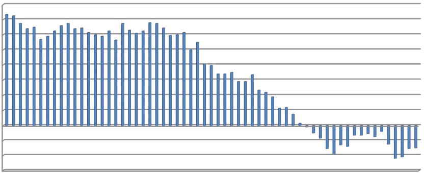
(Source: Bank of England; code: LPMVQJU)
However, private sector growth in the UK has remained weak, and the popular wisdom is that in part this weakness reflects inability of the private sector to access credit (at least at affordable interest rates). As highlighted in Figure 1, monthly growth rates in the lending component of M4 has declined steadily since the crisis, and has remained negative since Q3 of 2010-11. But, there is little evidence as yet about firm-level financing constraints. The contribution of this paper is to examine the empirical evidence of financing constraints among a cross-section of firms in the UK, to inform the debate about credit market failures in the post-recession period.
Specifically, we use make use of stylised as well relatively new methodologies to examine the extent of financing constraints among firms. Our results based on the stylised approach, which relates the cash flow sensitivity of investment to financing constraints in firms, suggests that, contrary to popular wisdom, the average firm in our sample does not experience financing constraint; during the crisis years, cash flow sensitivity of investment was negative. We then use a (relatively new) stochastic frontier approach to estimate the efficiency with which firms are able to translate their sales figures into investment, after controlling for year- (or financial crisis) and industry-specific shocks. The measure of investment efficiency has a lower bound of 0 and an upper bound of 1. Firms that do not experience significant frictions in credit and capital markets should have an investment efficiency level close to 1, while those that experience significant frictions in these markets will have considerably lower values of investment efficiency. Our results indicate that there is considerable heterogeneity in investment efficiency across firms, during a given year; the range being 0.57-0.82. However, the average investment efficiency measure is similar across years, regions and NACE 2-digit industries. We also do not find discernible patterns in the relationship between investment efficiency and firm size, both before and during the financial crisis. The results suggest that while some firms are clearly less efficient at translating their performance into investment, broad policies targeting firms of a certain size, or those within a particular industry or region, may not successfully address the problem of financing constraint in the United Kingdom. The targeting of firms with financing constraints may have to be considerably more refined.
The rest of the paper is structured as follows: In Section 2, we discuss the empirical strategy, and the data. The regression results are reported and discussed in Section 3. Finally, Section 4 concludes.
2. Empirical strategy and data
2.1 Stylised approach to modelling financing constraint
Following the arguments of James Tobin, it is stylised that in a world without capital market imperfections and taxes, the investment of a firm that maximises its net worth will depend on its Tobin's q (Yoshikawa, 1980). The "q" theory posits that if a firm's investment strategies are fundamentally sound then investors' valuation of the firm would be higher than the cost of the assets required to undertake production. Hence, if a firm's q the ratio of the market value of its assets to the replacement cost of these assets is greater than 1 then the firm would be encouraged to invest further, while a value of q that is less than 1 would discourage investment.
This basic model about the determinant of investment has been extended in a number of ways. To begin with, recent studies have taken into consideration the possibility that investment decisions may be affected by the demand for a firm's output. In such cases, there is a departure from Hayashi's (1982) argument that under plausible circumstances the marginal q used in Tobin's analysis and the more readily observable average q are identical; investment depends on output as well. Not surprisingly perhaps, early attempts at empirical estimation of investment functions find that, along with (average) q, the output level of firms have statistically significant coefficients (Abel, 1980). This statistically significant relationship is confirmed by more recent studies (Blundell et al., 1992; Cuthbertson and Gasparro, 1995).
It was further recognised that since capital markets are prone to failures on account of informational imperfections (Stiglitz and Weiss, 1981), it is important to take into account the factors that determine whether or not a firm is finance constrained. Initially, the literature focussed on the internal resources of the firms, with cash flows as a proxy for internal resources. Fazzari, Hubbard and Petersen (1988) include the firms' cash flows in the specification, and argue that a statistically significant (and positive) coefficient for the cash flow variable indicates the presence of financing constraints. In other words, the regression specification is given by
$$
\frac{I_{it}}{K_{i,t-1}} = f \left(\frac{X_{it}}{K_{i,t-1}} + g \frac{CF_{it}}{K_{i,t-1}}\right) + \epsilon_{it} \quad [1]
$$
where I is investment, X is vector of variables that captures investment opportunities, CF is cash flow, K is capital, and $\epsilon$ is the independently and identically distributed (i.i.d.) noise term. In the literature, this regression model has been estimated using both cross-section and panel data, with the latter facilitating control for firm- and year- fixed effects. The significance (and positive sign) of the coefficient for the cash flow variable (CF) indicates presence of financing constraints, and this is borne out by a number of empirical studies (e.g., Bond and Meghir, 1994; Devereux and Schiantarelli, 1990; Kadapakkam, Kumar and Riddick, 1998).
However, this approach has two significant shortcomings. First, the regression results indicate whether the average firm experiences financing constraint, thereby ignoring possible heterogeneity in the degree of financing constraints experienced by different types of firms. Second, it has been argued that the cash flow variable in the specification may not accurately capture the need for use of internal resources, and hence the extent of financing constraints (Kaplan and Zingales, 1997, 2000). If so, insignificance of the coefficient of the cash flow variable may not reflect absence of financing constraints, i.e., the null and alternative hypotheses that lie at the heart of the analysis may no longer be well defined. In the next section, therefore, we discuss an empirical strategy that helps overcome the shortcomings of the stylised approach.
2.2 Stochastic frontier based approach to modelling financing constraints
To reiterate, in the stylised literature that builds on the pioneering work of Fazzari, Hubbard and Petersen (1988), a firm's investment decisions depend only on its future prospect, which is captured by Tobin's q, and perhaps also by its current and past sales (the components of vector X in equation 1). If other firm characteristics such as cash flow have an impact on these investment decisions, the firm is believed to be financially constrained. In other words, in the absence of capital market imperfections and financing constraints, Tobin's q and current and past sales are sufficient to characterise the investment decisions of the firm.
In keeping with this, Wang (2003) and Bhaumik et al. (2012) argue that in the absence of agency conflicts and capital market imperfections a firm's investment decision can be defined as follows:
$$
\ln \left(\frac{I_{i,t}}{K_{i,t-1}}\right)^{SF} = \alpha + \beta \ln Q_{i,t} + \gamma \ln \left(\frac{SALE_{i,t}}{K_{i,t-1}}\right) + \delta \ln \left(\frac{SALE_{i,t-1}}{K_{i,t-2}}\right) + \theta_t + \mu_i + \epsilon_{it} \quad [2]
$$
where $\theta$ and $\mu$ capture time and firm (or industry) fixed effects, and $\epsilon$ is the i.i.d. error term. This regression model, therefore, defines the efficient investment function (frontier). In the presence of financing constraints, the observed investment-to-capital ratio is less than the efficient (optimal) investment-to-capital ratio in [2]. Thus, the difference between this efficient investment-to-capital ratio and the observed investment-to-capital ratio is attributed to financing constraint. This difference can be represented by a non-negative term u. More specifically, we write the observed investment-to-capital ratio as:
$$
\left(\frac{I_{i,t}}{K_{i,t-1}}\right) = \left(\frac{I_{i,t}}{K_{i,t-1}}\right)^{SF} \exp(-u_{it}) \implies \ln \left(\frac{I_{i,t}}{K_{i,t-1}}\right) = \ln \left(\frac{I_{i,t}}{K_{i,t-1}}\right)^{SF} - u_{it} \quad [3]
$$
Models [2] and [3] together define the stochastic frontier formulation of the investment function, and can be estimated using certain distributional assumptions on u and $\epsilon$. Specifically, $\epsilon$ is the normally distributed i.i.d. term, while u has a half normal distribution (Kumbhakar and Lovell, 2000).
It is evident that the stochastic frontier approach gives us not only the estimates of the parameters of the investment function but observation-specific estimates of the one-sided investment efficiency term u as well, and therein lies the key to the application of stochastic frontier approach to the literature on firm-level financing constraints. The higher the value of u greater is the impact of constraints on investment. Thus, in the present case, the frontier represents the desired investment function which is unobserved and the u term represents a firm's inability to attain the investment frontier, ceteris paribus, due to the presence of financing constraints. Specifically, from u, we are able to generate a score for investment efficiency, the equivalent of the technical efficiency measure for a production function (i.e., exp(-u$_{it}$)), which is bounded within (0, 1). Aside from the ease of interpretation – higher investment efficiency implies lower financing constraints, the investment efficiency score has the advantage that it captures the combined impact of all the constraining variables on the extent of credit constraint. By contrast, alternative methodologies such as OLS or fixed effects panel regression models captures only the marginal impact of individual firm characteristics on investment of the average firm, and hence do not tell us whether or not an individual firm is credit constrained overall, and if so by how much, relative to the frontier. With the stochastic frontier approach, therefore, it is possible to examine distributions of the extent of financing constraints of the firms from the efficiency scores, and compare distributions of financing constraints (or investment efficiency) across firm types, industries and regions, and over time.
2.3 Empirical strategy and data
Our analysis proceeds in two stages.
- First, we estimate variations of the stylised model outlined in equation [1] and examine the sign and significance of the coefficient of the cash flow variable. As mentioned above, a positive and significant estimate of this coefficient should indicate presence of financing constraints. We estimate equation [1] using both OLS and panel fixed effects models. In the case of the former, the standard errors are clustered to account for possible correlations of investment within firms over time. In order to distinguish between the pre-crisis period and the crisis period (2008-10), we include in the specifications of the OLS and fixed effects models both a dummy variable for the crisis years, and an interaction between this dummy variable and the cash flow variable.
- Next, we estimate the stochastic frontier models described by equations [2] and [3]. This enables us to generate measures of the efficiency with which firm characteristics such as current and past sales are translated into investment, and hence measures of financing constraints. Since these measures of financing constraints (alternatively, investment efficiency) are generated for all firm-years using the same frontier equation, we are able to compare these measures across industries and regions, as well as over time.
- Finally, under the restrictive assumption that growth in a certain period is indicative of growth in future periods, we examine how the investment efficiencies of firms in the four (sales) growth quartiles for the 2001-2003 period compare over the 2003-2010 period. In particular, we are interested in whether faster growing firms (i.e., those in the highest growth quartile during 2001-2003) experience greater financing constraints that other firms during the subsequent years.
For our analysis, we use firm level data from FAME, which is a much used source of firm level data for the UK. One of the weaknesses of FAME is that the data are self-reported and hence there is a high incidence of missing information for a large number of firms. In particular, data on Tobin's q are not available for more than 1000 firm-years. Hence, for the stochastic frontier part of our analysis, we have modelled investment-to-capital ratio of firms as a function of current and past sales alone:
$$
\ln \left(\frac{I_{i,t}}{K_{i,t-1}}\right)^{SF} = \alpha + \gamma \ln \left(\frac{SALE_{i,t}}{K_{i,t-1}}\right) + \delta \ln \left(\frac{SALE_{i,t-1}}{K_{i,t-2}}\right) + \theta_t + \mu_i + \epsilon_{it} \quad [2a]
$$
To begin with, we control for only the shock of the crisis years (2008-2010) using a dummy. Laterm we add controls for individual years and industries – initially NACE 2-digit and later NACE 4-digit – to account for time and industry fixed effects.
Table 1 Descriptive statistics
|
2003 |
2004 |
2005 |
2006 |
2007 |
2008 |
2009 |
2010 |
| Investment-to-capital ratio |
0.24 |
0.25 |
0.27 |
0.29 |
0.26 |
0.26 |
0.33 |
0.24 |
|
(0.22) |
(0.23) |
(0.24) |
(0.23) |
(0.24) |
(0.24) |
(0.21) |
(0.23) |
| Sales-to-capital ratio |
40.34 |
58.05 |
73.37 |
53.72 |
77.01 |
115.96 |
111.28 |
105.96 |
|
(662.06) |
(110.69) |
(624.21) |
(319.77) |
(925.14) |
(1122.36) |
(2897.89) |
(1835.44) |
| Cash flow-to-capital ratio |
1.34 |
2.10 |
2.40 |
2.55 |
3.80 |
3.98 |
3.77 |
3.17 |
|
(15.51) |
(18.30) |
(32.23) |
(27.54) |
(65.49) |
(62.74) |
(53.06) |
(33.72) |
| Fixed assets (£) |
20433.87 |
16583.55 |
12863.70 |
23658.52 |
16613.30 |
10224.27 |
22640.69 |
8312.52 |
|
(224009.20) |
(204269.60) |
(153357.20) |
(254512.60) |
(200041.70) |
(153724.60) |
(255965.60) |
(64683.02) |
| No. of obs. |
15480 |
13730 |
12983 |
18654 |
15186 |
11693 |
18792 |
8351 |
Notes: This table reports the means and standard deviations of the variables used for the analysis. The latter are reported within parentheses.
3. Regression results
In Table 2, we report the results for the stylised model (equation [1]). We estimate the model using both OLS with clustered standard errors to account for correlations within firms across years, and panel fixed effects. We estimate the model with the basic specification in which investment is determined by sales (models 1 and 4), the extended and (from our point of view) the extended model that includes cash flow and (log) assets (models 2 and 5), and a further extension in which the specification includes a dummy for the crisis years (2008-2010) and an interaction between this dummy and cash flows (models 3 and 6). The intuition for models 3 and 6 is that cash flow sensitivity of investment might differ significantly between pre-crisis and crisis years. From the point of view of signs and statistical significance of the estimated coefficients, the results are remarkably robust across specifications and estimation methods.
Table 2 Stylised regression models
|
OLS with clustered std. error |
|
|
Fixed effects |
|
|
|
Model 1 |
Model 2 |
Model 3 |
Model 4 |
Model 5 |
Model 6 |
| Sales-to-capital ratio |
0.06 *** |
0.07 *** |
0.07 *** |
0.14 *** |
0.25 *** |
0.25 *** |
|
(0.00) |
(0.00) |
(0.00) |
(0.00) |
(0.00) |
(0.00) |
| Lagged sales-to-capital ratio |
-0.02 *** |
- 0.02 *** |
- 0.02 *** |
- 0.01 |
- 0.02 *** |
- 0.02 *** |
|
(0.00) |
(0.00) |
(0.00) |
(0.00) |
(0.00) |
(0.00) |
| Cash flow-to-capital ratio |
|
- 0.0001 *** |
- 0.00001 |
|
- 0.0003 *** |
- 0.0001 ** |
|
|
(0.00) |
(0.00) |
|
(0.00) |
(0.00) |
| (Log) fixed assets |
|
0.005 *** |
0.005 *** |
|
0.13 *** |
0.13 *** |
|
|
(0.00) |
(0.00) |
|
(0.00) |
(0.00) |
| Crisis year dummy |
|
|
0.01 *** |
|
|
- 0.001 |
|
|
|
(0.00) |
|
|
(0.00) |
| Crisis year dummy × Cash flow-to-capital |
|
|
- 0.0001 *** |
|
|
- 0.0002 *** |
|
|
|
(0.00) |
|
|
(0.00) |
| Constant |
0.16 *** |
0.11 *** |
0.11 *** |
- 0.05 *** |
- 1.21 *** |
- 1.21 *** |
|
(0.00) |
(0.00) |
(0.00) |
(0.00) |
(0.01) |
(0.01) |
| No. of observations |
114861 |
114861 |
114861 |
114861 |
114861 |
114861 |
| Number of firms |
36934 |
36934 |
36934 |
36934 |
36934 |
36934 |
| F-statistics |
3234.47 *** |
1634.60 *** |
1119.63 *** |
3848.45 *** |
3796.80 *** |
2536.75 *** |
| R-squared |
0.08 |
0.08 |
0.08 |
0.07 |
0.02 |
0.02 |
Notes: This table reports the estimates of the stylised regression model (equation [1]). The values within parentheses are standard errors. *** indicates significance at the 1 percent levels. For fixed effect models, we report the overall R-square. In this model, the average firm in the sample is considered to be experiencing financing constraint if the coefficient of the cash flow variable is positive and significant. In the case of our sample, this coefficient is either insignificant or negative, for both the pre-crisis and crisis years. In other words, our regression results do not indicate presence of financing constraint for the average firm for either the pre-crisis or the crisis years.
To recapitulate, in this stylised approach, the average firm is said to experience financing constraints if the coefficient of the cash flow variable is positive and significant. The results reported in the table suggest that the average firm in the sample did not experience financing constraint during the sample period; the estimated coefficient of the cash flow variable is negative. Indeed, while the cash flow sensitivity of investment during the crisis years was different compared to that in pre-crisis years, the sensitivity was even more negative during the former. The coefficients of the other variables are consistent with expectations (see Bhaumik et al., 2012): current sales and investment are positively related while past sales and investment have a negative relationship, and investment-to-capital ratio is higher for larger firms. Importantly, the dummy for the crisis years does not have a significant coefficient, indicating that there was no secular impact of the crisis on the investment-to-capital ratio of the firms in the sample. This is consistent with the cross-year values of the average investment-to-capital ratio reported in Table 1.
Table 3 Investment efficiency - frontier equation
|
Model 1 |
Model 2 |
Model 3 |
Model 4 |
| Sales(t)/Capital(t-1) |
0.069 *** |
0.069 *** |
0.073 *** |
0.074 *** |
|
(0.001) |
(0.001) |
(0.001) |
(0.001) |
| Sales(t-1)/Capital(t-2) |
- 0.026 *** |
- 0.026 *** |
- 0.028 *** |
- 0.028 *** |
|
(0.001) |
(0.001) |
(0.001) |
(0.001) |
| Crisis dummy |
|
0.015 *** |
|
|
|
|
(0.001) |
|
|
| Constant |
0.661 |
0.655 |
0.634 |
0.614 |
|
(8.097) |
(7.611) |
(4.85) |
(7.585) |
| Year dummies |
No |
No |
Yes |
Yes |
| Industry dummies |
No |
No |
No |
Yes |
| Log likelihood |
8451.84 |
8512.71 |
9746.42 |
10305.54 |
| Wald chi-square |
8759.43 *** |
8901.67 *** |
11447.51 *** |
12839.07 *** |
| Gamma |
0.113 |
0.113 |
0.127 |
0.113 |
|
(0.030) |
(0.003) |
(0.003) |
(0.003) |
| Number of firms |
36934 |
36934 |
36934 |
36721 |
| Number of obs. |
114861 |
114861 |
114861 |
113764 |
Notes: This table reports the estimates of the stochastic frontier model (equation [2a]). The values within parentheses are standard errors. *** indicates significance at the 1% level. Models 3 and 4 control for NACE 2-digit industry fixed effects. Theoretically, for a frontier to exist, gamma should have a value between zero and one. On the basis of these estimates, we generate firm-year specific estimates of investment efficiency which lies between 0 and 1. If the investment efficiency of a firm is close to 1 then it experiences very little financing constraint, and vice versa.
Next, we estimate the stochastic frontier model outlined in equation [2a]. The regression estimates are reported in Table 3. We report the estimates for four different specifications: the basic specification in which investment is determined by sales (model 1), one in which we control for the crisis years (model 2), one in which we control for unobserved year effects (model 3), and finally one in which we control for both unobserved year and (NACE 2-digit) industry effects. As discussed earlier in the paper, stochastic frontier analysis generates a firm-year specific (0, 1) bounded measure of investment efficiency; financing constraint decreases with this efficiency measure.
Investment efficiency in manufacturing (Alternative specifications)
Descriptive plot of investment efficiency, with a peak around 0.7-0.8, showing distributions for basic specification, specification with a crisis dummy, specification with year dummies, and specification with year and industry dummies.
| Descriptive statistics |
Model 1 |
Model 2 |
Model 3 |
Model 4 |
| Model 1 |
0.716 |
1.00 |
|
|
|
(0.042) |
|
|
|
| Model 2 |
0.716 |
0.99 |
1.00 |
|
|
(0.042) |
|
|
|
| Model 3 |
0.717 |
0.99 |
0.99 |
1.00 |
|
(0.045) |
|
|
|
| Model 4 |
0.721 |
0.98 |
0.98 |
0.98 |
|
(0.041) |
|
|
1.00 |
Notes: The values within parentheses are standard deviations of the investment efficiency estimates generated from the stochastic frontier models (Table 3). The values in columns 2-5 are correlation coefficients. Since the correlation among the investment efficiency estimates generated by the four models is high, we can use any one of these measures for our analysis. For the rest of the analysis, therefore, we use the estimates of investment efficiency generated by Model 1.
In Table 4, we report the means, standard deviations, and maximum and minimum values for investment efficiency across years. The descriptive statistics suggest that the average values of the efficiency measure were quite similar across the years – if anything, average efficiency actually increased during 2009 and 2010. Note that our estimates of investment efficiency is based on firm-year observations for the entire 2003-2010 period, i.e., these estimates are based on the same underlying efficient frontier. Under the reasonable assumption that firms did not, on average, experience significant financing constraint during the pre-crisis years, the observation that investment efficiency (and hence the degree of financing constraint) is similar for the pre-crisis and crisis years, is consistent with the result from the stylised model, namely, that there is no financing constraint for the average firm in the sample. The descriptive statistics also indicate that there is considerable variation in the efficiency measure across firms, during each of the years in the sample period. The efficiency measure ranged from 0.57 to 0.82 for all these years.
Table 4 Investment efficiency across time
|
Number of observations |
Mean |
Standard Deviation |
Maximum |
Minimum |
| 2003 |
15480 |
0.713 |
0.039 |
0.575 |
0.819 |
| 2004 |
13730 |
0.708 |
0.039 |
0.575 |
0.823 |
| 2005 |
12983 |
0.708 |
0.040 |
0.575 |
0.823 |
| 2006 |
18654 |
0.717 |
0.040 |
0.575 |
0.822 |
| 2007 |
15186 |
0.713 |
0.041 |
0.575 |
0.822 |
| 2008 |
11693 |
0.716 |
0.044 |
0.575 |
0.823 |
| 2009 |
18792 |
0.726 |
0.044 |
0.575 |
0.822 |
| 2010 |
8351 |
0.724 |
0.049 |
0.575 |
0.818 |
Notes: This table reports the descriptive statistics for the estimates of investment efficiency across years. The average values of the efficiency measure were quite similar across the sample years – if anything, average efficiency actually increased during 2009 and 2010. Under the reasonable assumption that firms did not, on average, experience significant financing constraint during the pre-crisis years, the observation that investment efficiency (and hence the degree of financing constraint) is similar for the pre-crisis and crisis years, it is possible to argue that there is no financing constraint for the average firm in the sample. The range of values for investment efficiency also indicate that there is considerable variation in the efficiency measure across firms, during each of the years in the sample period.
Next, we examine whether there is noticeable variation in the average measure of investment efficiency across 2-digit industries and regions. In Table 5, we report the average value of the estimated investment efficiency across regions in the United Kingdom, and across years. In Table 6, we report the average value of the efficiency measure across 2-digit industries, and across years. Since an average is not a meaningful statistic for very small samples, in Table 6, we report average values of investment efficiency for only those 2-digit industries for which we have at least 10 firms for all (or most) of the years. The averages reported in Table 5 indicate that average investment efficiency of firms was fairly similar across regions, and remarkably stable over the years. Importantly, there was no noticeable decline in average investment efficiency during the crisis years in any of the years; average investment efficiency was marginally above trend in 2009 and 2010. Similarly, the averages for the industry-years reported in Table 6 indicate that while there are modest inter-industry differences in average investment efficiency for any given year, and modest differences in average efficiency for any one industry across years, the differences are not significant.
Table 5 Investment efficiency across regions
|
2003 |
2004 |
2005 |
2006 |
2007 |
2008 |
2009 |
2010 |
| East Midlands |
0.706 |
0.699 |
0.699 |
0.708 |
0.704 |
0.704 |
0.718 |
0.720 |
| East of England |
0.711 |
0.705 |
0.703 |
0.712 |
0.709 |
0.713 |
0.722 |
0.720 |
| London |
0.716 |
0.713 |
0.715 |
0.722 |
0.719 |
0.723 |
0.732 |
0.725 |
| North East |
0.711 |
0.705 |
0.703 |
0.716 |
0.713 |
0.719 |
0.728 |
0.730 |
| North West |
0.710 |
0.704 |
0.706 |
0.715 |
0.711 |
0.711 |
0.725 |
0.723 |
| Northern Ireland |
0.716 |
0.709 |
0.705 |
0.715 |
0.708 |
0.715 |
0.728 |
0.751 |
| Scotland |
0.716 |
0.708 |
0.708 |
0.717 |
0.711 |
0.717 |
0.726 |
0.727 |
| South East |
0.712 |
0.707 |
0.707 |
0.716 |
0.712 |
0.716 |
0.724 |
0.720 |
| South West |
0.710 |
0.706 |
0.706 |
0.714 |
0.710 |
0.714 |
0.724 |
0.724 |
| Wales |
0.709 |
0.702 |
0.704 |
0.712 |
0.711 |
0.710 |
0.720 |
0.724 |
| West Midlands |
0.708 |
0.702 |
0.702 |
0.713 |
0.708 |
0.709 |
0.721 |
0.721 |
| Yorkshire & Humberside |
0.709 |
0.734 |
0.705 |
0.712 |
0.707 |
0.708 |
0.720 |
0.723 |
Notes: This table reports the average investment efficiency of firms for each region in each of the sample years. These numbers suggest that average investment efficiency of firms was fairly similar across regions, and remarkably stable over the years. Importantly, there was no noticeable decline in average investment efficiency during the crisis years in any of the years; average investment efficiency was marginally above trend in 2009 and 2010.
Table 6 Investment efficiency across 2-digit industries
|
2003 |
2004 |
2005 |
2006 |
2007 |
2008 |
2009 |
2010 |
| 1 |
0.714 |
0.702 |
0.698 |
0.714 |
0.705 |
0.705 |
0.721 |
0.731 |
| 11 |
0.716 |
0.718 |
0.724 |
0.725 |
0.730 |
0.735 |
0.739 |
0.729 |
| 14 |
0.713 |
0.709 |
0.704 |
0.713 |
0.711 |
0.709 |
0.716 |
0.712 |
| 15 |
0.696 |
0.696 |
0.692 |
0.701 |
0.692 |
0.694 |
0.708 |
0.712 |
| 17 |
0.702 |
0.702 |
0.698 |
0.717 |
0.701 |
0.689 |
0.712 |
0.723 |
| 18 |
0.698 |
0.698 |
0.699 |
0.705 |
0.690 |
0.689 |
0.697 |
0.717 |
| 19 |
0.695 |
0.695 |
0.691 |
0.696 |
0.705 |
0.693 |
0.700 |
0.712# |
| 20 |
0.696 |
0.696 |
0.692 |
0.702 |
0.694 |
0.684 |
0.720 |
0.718 |
| 21 |
0.704 |
0.704 |
0.703 |
0.711 |
0.699 |
0.696 |
0.718 |
0.717 |
| 22 |
0.708 |
0.708 |
0.709 |
0.713 |
0.707 |
0.705 |
0.718 |
0.718 |
| 23 |
0.691 |
0.691 |
0.687# |
0.702 |
0.688 |
0.670 |
0.718 |
0.705# |
| 24 |
0.699 |
0.698 |
0.696 |
0.707 |
0.698 |
0.701 |
0.714 |
0.711 |
| 25 |
0.703 |
0.703 |
0.697 |
0.706 |
0.699 |
0.691 |
0.712 |
0.707 |
| 26 |
0.704 |
0.704 |
0.701 |
0.707 |
0.697 |
0.696 |
0.713 |
0.716 |
| 27 |
0.695 |
0.695 |
0.687 |
0.700 |
0.695 |
0.698 |
0.705 |
0.703 |
| 28 |
0.696 |
0.695 |
0.695 |
0.707 |
0.699 |
0.695 |
0.711 |
0.715 |
| 29 |
0.695 |
0.695 |
0.694 |
0.703 |
0.700 |
0.701 |
0.713 |
0.712 |
| 30 |
0.711 |
0.711 |
0.715 |
0.712 |
0.709 |
0.706 |
0.715 |
0.711 |
| 31 |
0.699 |
0.698 |
0.697 |
0.704 |
0.700 |
0.702 |
0.711 |
0.712 |
| 32 |
0.699 |
0.699 |
0.699 |
0.704 |
0.702 |
0.700 |
0.709 |
0.708 |
| 33 |
0.702 |
0.702 |
0.704 |
0.709 |
0.705 |
0.707 |
0.720 |
0.713 |
| 34 |
0.695 |
0.695 |
0.688 |
0.698 |
0.695 |
0.697 |
0.708 |
0.693 |
| 35 |
0.697 |
0.696 |
0.699 |
0.705 |
0.703 |
0.697 |
0.714 |
0.694 |
| 36 |
0.699 |
0.699 |
0.698 |
0.706 |
0.699 |
0.698 |
0.711 |
0.719 |
| 37 |
0.707 |
0.706 |
0.712 |
0.714 |
0.723 |
0.737 |
0.748 |
0.760 |
| 40 |
0.707 |
0.706 |
0.715 |
0.731 |
0.721 |
0.727 |
0.739 |
0.720 |
| 41 |
0.725 |
0.709# |
0.709# |
0.727 |
0.716 |
0.727 |
0.726 |
|
| 45 |
0.703 |
0.703 |
0.702 |
0.709 |
0.707 |
0.706 |
0.717 |
0.724 |
| 50 |
0.702 |
0.701 |
0.697 |
0.708 |
0.698 |
0.699 |
0.714 |
0.712 |
| 51 |
0.699 |
0.699 |
0.698 |
0.706 |
0.700 |
0.702 |
0.712 |
0.717 |
| 52 |
0.707 |
0.707 |
0.708 |
0.716 |
0.712 |
0.715 |
0.724 |
0.712 |
| 55 |
0.713 |
0.713 |
0.715 |
0.729 |
0.717 |
0.721 |
0.737 |
0.728 |
| 60 |
0.706 |
0.706 |
0.705 |
0.711 |
0.707 |
0.704 |
0.715 |
0.723 |
| 61 |
0.712 |
0.712 |
0.716 |
0.730 |
0.728 |
0.738 |
0.741 |
0.717 |
| 62 |
0.713 |
0.712 |
0.714 |
0.721 |
0.719 |
0.721 |
0.723 |
0.717# |
| 63 |
0.705 |
0.704 |
0.701 |
0.709 |
0.704 |
0.706 |
0.718 |
0.706 |
| 64 |
0.726 |
0.725 |
0.727 |
0.727 |
0.729 |
0.733 |
0.735 |
0.724 |
| 65 |
0.720 |
0.720 |
0.721 |
0.728 |
0.725 |
0.729 |
0.737 |
0.730 |
| 66 |
0.719 |
0.719 |
0.722 |
0.723 |
0.722 |
0.723 |
0.738 |
0.725 |
| 67 |
0.723 |
0.723 |
0.723 |
0.732 |
0.729 |
0.732 |
0.742 |
0.734 |
| 70 |
0.723 |
0.722 |
0.725 |
0.737 |
0.727 |
0.732 |
0.747 |
0.733 |
| 71 |
0.713 |
0.713 |
0.710 |
0.714 |
0.713 |
0.712 |
0.723 |
0.725 |
| 72 |
0.721 |
0.721 |
0.723 |
0.727 |
0.726 |
0.729 |
0.733 |
0.731 |
| 73 |
0.726 |
0.726 |
0.723 |
0.731 |
0.732 |
0.730 |
0.737 |
0.739 |
| 74 |
0.715 |
0.715 |
0.716 |
0.724 |
0.724 |
0.728 |
0.737 |
0.734 |
| 75 |
0.725 |
0.725 |
0.723 |
0.736 |
0.739 |
0.739 |
0.745 |
0.746# |
| 80 |
0.718 |
0.718 |
0.716 |
0.722 |
0.717 |
0.723 |
0.727 |
0.732 |
| 85 |
0.714 |
0.714 |
0.715 |
0.728 |
0.724 |
0.725 |
0.740 |
0.732 |
| 90 |
0.712 |
0.711 |
0.710 |
0.714 |
0.714 |
0.720 |
0.728 |
0.751 |
| 91 |
0.720 |
0.720 |
0.726 |
0.730 |
0.727 |
0.728 |
0.734 |
0.727 |
| 92 |
0.715 |
0.715 |
0.713 |
0.722 |
0.718 |
0.723 |
0.729 |
0.723 |
| 93 |
0.712 |
0.711 |
0.708 |
0.721 |
0.715 |
0.717 |
0.729 |
0.729 |
Notes: This table reports the average investment efficiency of firms for a number of NACE 2-digit industries, in each of the sample years. The # sign indicates that the sample has fewer than 10 firms. The numbers indicate that while there are modest inter-industry differences in average investment efficiency for any given year, and modest differences in average efficiency for any one industry across years, the differences are not significant.
Finally, in Table 7, we explore the relationship between firm growth and investment efficiency. Since contemporaneous growth rates of firms are almost certainly endogenous to the extent of financing constraints, we focus on the growth rates of firms for the 2001-2003 period, the first three years for which data are available for a reasonably large sample of firms. We then separate the firms into four quartiles, on the basis of their 2001-2003 growth rates. High growth firms are likely to roughly correspond to the firms in the highest growth quartile (quartile 4). As before, we report the average investment efficiencies for the firms in the four quartiles for each of the years in the sample period. Since we have an unbalanced panel, and not all firms for which we can compute the growth rate for the 2001-2003 period are present in the sample for each of the years, for the sake of completeness we also report the average efficiency measure for these other firms. We notice two things: First, for each of the years, average investment efficiency is marginally higher for the fastest and slowest growing firms in the 2001-2003 cohort, than for the firms with intermediate rates of growth. It is reasonable to speculate therefore that the future growth of these latter firms, which are potentially high growth firms of the future, might find their growth restrained on account of financing constraint. Second, average investment efficiency of firms in the 2001-2003 cohort decrease over time, for all quartiles, even as there is an increase in the average efficiency of the other firms.
Table 7 Investment efficiency across 2003 growth quartiles
|
Quartile 1 |
Quartile 2 |
Quartile 3 |
Quartile 4 |
Others |
| 2003 |
0.721 |
0.710 |
0.712 |
0.722 |
0.711 |
| 2004 |
0.713 |
0.701 |
0.703 |
0.717 |
0.710 |
| 2005 |
0.709 |
0.696 |
0.699 |
0.715 |
0.713 |
| 2006 |
0.711 |
0.703 |
0.704 |
0.716 |
0.724 |
| 2007 |
0.703 |
0.693 |
0.696 |
0.709 |
0.710 |
| 2008 |
0.705 |
0.690 |
0.692 |
0.705 |
0.726 |
| 2009 |
0.707 |
0.699 |
0.701 |
0.712 |
0.736 |
| 2010 |
0.690 |
0.681 |
0.687 |
0.702 |
0.736 |
Notes: This table reports the average investment efficiency of firms for the four growth quartiles. The quartiles refer to the quartiles of 3-year (2001-2003) average of firm growth in 2003. Others refer to firms that were not in the 2003 cohort. The numbers suggest that, for each of the years, average investment efficiency is marginally higher for the fastest and slowest growing firms in the 2001-2003 cohort, than for the firms with intermediate rates of growth. It is reasonable to speculate therefore that the future growth of these latter firms, which are potentially high growth firms of the future, might find their growth restrained on account of financing constraint. Further, average investment efficiency of firms in the 2001-2003 cohort decrease over time, for all quartiles, even as there is an increase in the average efficiency of the other firms.
Taken together, the results suggest that the degree of financing constraint experienced by the average British firm was not significantly different between the pre-crisis years and the crisis years of 2008-2010. The average investment efficiency measure has a value of about 0.70 across years, across industries and across regions. This estimate of investment efficiency itself does not permit us to make an absolute statement about whether or not a the average firm was financially constrained. However, as we have argued earlier, under the reasonable assumption that the average firm did not experience financing constraint during the pre-crisis years, our results suggest that there is no prima facie evidence of significant financing constraint among British firms during the 2003-2010 period – importantly not even during the crisis years of 2008-2010, on average. However, as noted above, the distributions of investment efficiency suggest that there are considerable variations in this efficiency across firms during any one year. We interpret this as suggesting that policies aimed at alleviating financing constraints in firms would not be useful if they target broad categories such as firms in certain industries or within certain regions. The extent of financing constraints is likely driven by firm-specific factors that may or may not vary systematically with the measure of investment efficiency.
Four scatter plots illustrating the relationship between fixed assets and investment efficiency for UK firms.
The top-left plot shows "Scatter plot of fixed assets against investment efficiency (All firms (2003))".
The top-right plot shows "Scatter plot of fixed assets against investment efficiency (Smaller firms (2003))".
The bottom-left plot shows "Scatter plot of fixed assets against investment efficiency (All firms (2010))".
The bottom-right plot shows "Scatter plot of fixed assets against investment efficiency (Smaller firms (2010))".
Notes: In this figure, we report the scatter plots of the investment efficiency and fixed assets of firms, for 2003 (the first and pre-crisis year) and 2010 (the last and crisis year). In the graphs to the left, we include all firms in the sample, for the respective years. In the graphs to the right, we restrict the sample to firms with less than £500,000 in assets. In either case, there is no discernible pattern for the relationship between firm size and investment efficiency. Hence, even when targeting policies based on firm characteristics, policy makers may have to look beyond obvious (and easily observable) characteristics such as size.
As in the case of any empirical analysis, our results are subject to two important caveats. First, on account of paucity of data for Tobin's q, we were not able to include it in our regression specification. Hence, even though we control for unobserved industry-specific factors, our specification s may lack a forward-looking component. Second, once missing data etc are taken into account, we have a sample that accounts for 10 percent (or fewer) firms of the FAME population. Hence, the distribution of our sample across industries, firm sizes etc may not be representative of the respective distributions for the underlying population of firms in the United Kingdom. However, our results provide important evidence about the extent of financing constraints among British firms across a wide range of industries and over a number of years. Importantly, we are able to provide a comparable measure of this constraint (via investment efficiency) across firm-years. Further, the result about the absence of significant financing constraint for the average firm is remarkably consistent across choice of methodologies and specifications. Also, the key insight that financing constraints in firms may be driven largely by firm-specific factors such as credit risk and organisational capacity that are not easily observed is consistent with other available evidence on financing constraints of British firms. This gives us confidence about broad implications of our results, discussed above.
4. Conclusion
Inadequate access to financial resources is viewed as an impediment to growth of firms, and a popular view is that financing constraint is adversely affecting growth of firms (and the private sector) in the United Kingdom. In this paper, we address this policy issue using a stylised methodology that relies on estimates of the cash flow sensitivity of firms' investment, as well as a relatively new methodology that enables us to generate a measure of investment efficiency of firms, i.e., the efficiency with which firms can convert their sales into investment, after controlling for unobserved year- and industry-specific effects. This measure of investment efficiency, which is bounded between 0 and 1, permits us to compare the extent of financing constraints across firm-years, and hence across time, industries and regions.
Our results indicate that there is considerable heterogeneity in investment efficiency across firms, during a given year; the range being 0.57-0.82. However, the average investment efficiency measure is similar across years, regions and NACE 2-digit industries. We also do not find discernible patterns in the relationship between investment efficiency and firm size, both before and during the financial crisis. The results suggest that while some firms are clearly less efficient at translating their performance into investment, broad policies targeting firms of a certain size, or those within a particular industry or region, may not successfully address the problem of financing constraint in the United Kingdom. The targeting of firms with financing constraints may have to be considerably more refined, and look at not easily observable factors such as credit history/events and organisational capacity of the firms.
Our results should be interpreted with care. On account of the quality of available data, we were not able to fully use the stylised specification – specifically, include Tobin's q in the specification – and the distributions of the sample we use may not be representative of the distributions of the underlying firm population. But our results are robust. Further, the regression estimates and the key insight about the importance of not easily observable factors are consistent with the literature on financing constraints and other available evidence on financing constraints of British firms. Hence, our results should provide a strong basis for further (and perhaps more refined) policy debate about financing constraints of firms in the United Kingdom.
References
- Abel, A. (1980). Empirical investment equations: An integrative approach, Carnegie-Rochester Conference Series on Public Policy, 12(1): 39-91.
- Abel, A., Blanchard, O. (1989). Investment and sales: Some empirical evidence, Working paper no. 2050, National Bureau of Economic Research, Cambridge, Massachusetts.
- Allayannis, G., Mozumdar, A. (2004). The impact of negative cash flow and influential observations on investment – cash flow sensitivity estimates. Journal of Banking and Finance, 28(6): 901-930.
- Almeida, H., Campello, M., Weisbach, S. (2004). The cash flow sensitivity of cash. Journal of Finance, 59(4): 1777-1804.
- BDRC Continental (2012). SME Finance Monitor, Q1 2012: How has 2012 started? An independent report by BDRC Continental, May 2012.
- Bhaumik, S.K., Das, P., Kumbhakar, S.C. (2012). A stochastic frontier approach to modelling financial constraints in firms: An application to India. Journal of Banking and Finance, 36(5): 1311-1319.
- Blundell, R. et al. (1992). Investment and Tobin's Q, Journal of Econometrics, 51: 233-257.
- Bond, S. and Meghir, C. (1994). Dynamic investment models and the firm's financial policy, Review of Economic Studies, 61(2): 197-222.
- Cecchetti, S.G., Mohanty, M.S., Zampolli, F. (2011). The real effects of debt. Mimeo, Bank for International Settlements, Downloadable from http://www.bis.org/publ/othp16.pdf.
- Cuthbertson, K. and Gasparro, D. (1995). Fixed investment decisions in UK manufacturing: The importance of Tobin's Q, output and debt, European Economic Review, 39: 919-941.
- Devereux, S. and Schiantarelli, F. (1990). Investment, Financial Factors and Cash Flow: Evidence from UK Panel Data, In: R. Glenn Hubbard (Ed.),. Asymmetric Information, Corporate Finance and Investment,, Chicago: University of Chicago Press, pp. 279-306.
- Elmeskov, J., Sutherland, D. (2012). Post-crisis debt overhand: growth implications across countries. Mimeo, Organisation for Economic Cooperation and Development (OECD), Downloadable from http://www.oecd.org/dataoecd/7/2/49541000.pdf.
- Fazzari, S.M., Hubbard, R.G. and Petersen, B.C. (1988). Financing constraints and corporate investment, Brookings Papers on Economic Activity, Vol. 1, pp. 141-206.
- Fazzari, F., Petersen, B.C. (1993). Working capital and fixed investment: New evidence on financing constraints. RAND Journal of Economics, 24: 328-341.
- Hayashi, F. (1982). Tobin's marginal-Q and average-Q: A neoclassical interpretation, Econometrica, 50(1): 213-224.
- Hubbard, R.G. (1998). Capital market imperfections and investment. Journal of Economic Literature, 36: 193-225.
- Kadapakkam, P-R., Kumar, P.C. and Riddick, L.A. (1998). The impact of cash flows and firm size on investment: The international evidence, Journal of Banking and Finance, 22: 293-320.
- Kaplan, S.N., Zingales, L. (1997). Do investment-cash flow sensitivities provide useful measures of financing constraints? Quarterly Journal of Economics, 112(1): 169-215.
- Kaplan, S.N., Zingales, L. (1997). Investment-cash flow sensitivities are not valid measures of financing constraints? Quarterly Journal of Economics, 115(2): 707-712.
- Kumbhakar, S.C., Lovell, C.K.A. (2000). Stochastic frontier analysis. Cambridge University Press.
- Reinhart, C.M., Rogoff, K.S. (2011). A decade of debt. Working paper no. 16827, National Bureau of Economic Research, Cambridge, Massachusetts.
- Stiglitz, J.E., Weiss, A.M. (1981). Credit rationing in markets with imperfect competition. American Economic Review, 71: 393-410.
- Wang, H-J., 2003. A stochastic frontier analysis of financing constraints on investment: The case of financial liberalization in Taiwan. Journal of Business and Economic Statistics 21, 406-419.
- Yoshikawa, H. (1980). On the "q" theory of investment, American Economic Review, 70(4): 739-743.